Hindawi Publishing Corporation International Journal of Distributed Sensor Networks Volume 2016, Article ID 8527312, 12 pages http://dx.doi.org/10.1155/2016/8527312
Research Article Unbalanced Threshold Based Distributed Data Collection Scheme in Multisink Wireless Sensor Networks Guorui Li,1 Ying Wang,2 Cong Wang,1 and Yiying Liu1 1
College of Information Science and Engineering, Northeastern University, Shenyang, Liaoning 110819, China Department of Information Engineering, Qinhuangdao Institute of Technology, Qinhuangdao, Hebei 066100, China
2
Correspondence should be addressed to Guorui Li;
[email protected] Received 18 September 2015; Revised 19 November 2015; Accepted 1 December 2015 Academic Editor: Yao Liang Copyright © 2016 Guorui Li et al. This is an open access article distributed under the Creative Commons Attribution License, which permits unrestricted use, distribution, and reproduction in any medium, provided the original work is properly cited. In multisink wireless sensor networks, synchronized data collection among multiple sinks is a significant and challenging task. In this paper, we propose an unbalanced threshold based distributed data collection scheme to reconstruct the synchronized sensed data of the whole sensor network in all sinks. The proposed scheme includes the unbalanced threshold based distributed top-|𝐾| query algorithm and the distributed iterative hard thresholding algorithm. By computing unbalanced thresholds and pruning unnecessary element exchanging, each sink can synchronize the top-|𝐾| aggregated values efficiently via the unbalanced threshold based distributed top-|𝐾| query algorithm. After that, the synchronized sensed data of the whole sensor network can be reconstructed through the distributed iterative hard thresholding algorithm in a distributed and cooperative manner. We show through experiments that the proposed scheme can reduce the interaction times and decrease the number of transmitted data and that of computed data compared to the existing schemes while maintaining the similar data reconstruction accuracy. The communication and computational performances of the proposed scheme are also analyzed in detail in the paper.
1. Introduction Wireless sensor network (WSN) is an autonomous wireless network consisting of a large number of tiny, inexpensive, and spatially distributed wireless sensor nodes. It has emerged as one of the most promising technologies for the future [1]. The typical applications of WSN include environment monitoring, industrial process control, intelligent transportation, military surveillance, and health care monitoring [2]. However, wireless sensor nodes have severe resource constraints which include limited computational, memory, communication capacities and nonrenewable energy supply. Therefore, data collection schemes in wireless sensor network should be light weight and energy efficient. Two representative types of data collection schemes in wireless sensor networks are spatial-temporal correlation based data predication schemes [3–5] and distributed source coding schemes [6–8]. In the first type of data collection scheme, a series of spatialtemporal correlation based data prediction algorithms are adopted to prolong the system lifetime by enabling the sink to predict the sensed data based on some historical samples.
In the second type of data collection scheme, distributed source coding techniques, such as Slepian-Wolf coding and Wyner-Ziv coding, are designed to compress the multiple correlated sensor data without the need of communication among sensor nodes. Nevertheless, the computational and communication cost of the above two types of data collection schemes are still high. Meanwhile, the parameters of predication model and the distributed coded data are still required to be computed and transmitted within the network frequently. Recently, compressive sensing (CS) theory has attracted considerable attention in areas of signal processing, computer science, and applied mathematics [9]. It is based on the principle that a sparse signal can be reconstructed from far fewer samples than that required by the classic ShannonNyquist sampling theory. Through nonlinear optimization, we can recover many natural signals which can be represented by a few nonzero coefficients under a suitable basis [10]. The inherent characteristics, such as compressibility, robustness, versatility, and stability, have made compressive sensing theory widely applied to communication [11], photography [12], magnetic resonance imaging [13], astronomy [14], and so forth.
2 As for the data collection problem in wireless sensor networks, a number of compressive sensing based schemes have been proposed in the literature. In 2009, Luo et al. proposed the first complete compressive sensing based data gathering (CDG) scheme for large scale wireless sensor networks [15]. By adapting a weighted sum of all the readings along the routing tree, CDG scheme can achieve substantial communication cost reduction and balanced energy consumption simultaneously. In order to achieve both energy efficiency and recovery fidelity, Xiang et al. proposed the Compressive Data Aggregation (CDA) scheme in WSN [16]. After abstracting the minimum energy compressed data aggregation problem as a NP-completeness problem, they solve it using a mixed integer programming formulation method. Moreover, they also proposed the Dual-lEvel Compressed Aggregation (DECA) framework to recover the in-network aggregated data in the widespread monitoring area by utilizing both the low-rank nature of real-world events and the redundancy in sensed data [17]. By exploiting the spatial and temporal correlation among sensed data, Xu et al. proposed the SpatioTemporal Hierarchical Data Aggregation Scheme Using Compressive Sensing (ST-HDACS) in [18]. After collecting the sensed data from a subset of randomly selected sensor nodes through a hierarchical routing structure, the fusion center recovers the whole sensed data by solving a matrix completing problem. Furthermore, Tang et al. proposed a robust compressive data gathering scheme to identify outlying sensor readings and derive the corresponding accurate values and further infer broken links in the sensor network [19]. Motivated by the fact that the variance among all the solutions of the blind iterative hard thresholding algorithm with different sparse level can indicate the best sparse level, Xiong and Tang proposed the blind 1-bit compressive sensing reconstruction algorithm for wireless sensor network [20]. Similar research works include the sparse random scheduling based data gathering scheme [21], the Resource Efficient Data Gathering (REDG) scheme [22], the Compressive Sensing Based Data Aggregation Scheme (CSDAS) [23], and the distributed multichain based compressive sensing scheme [24]. Although the above schemes can achieve energy-efficient data collection based on compressive sensing theory, they can only be applied to single-sink wireless sensor networks in a centralized manner. In the scenario of multisink wireless sensor networks, compressed data should be transmitted to one specific sink before executing the data reconstruction algorithm. Then, the recovered data should be distributed back to other sinks through unicast or broadcast messages. Obviously, this kind of centralized pattern is less energy efficient and time consuming. In this paper, we focus on designing compressive sensing based distributed data collection scheme for multisink wireless sensor networks. The proposed scheme includes two correlated algorithms: the unbalanced threshold based distributed top-|𝐾| algorithm and the distributed iterative hard thresholding algorithm. In the first algorithm, the largest 𝐾 absolute aggregated values of a series of object-value pairs are queried in a distributed and energy efficient way. By computing unbalanced thresholds, a number of unnecessary object-value pairs exchanging
International Journal of Distributed Sensor Networks are pruned in the query process. In the second algorithm, the iterative hard thresholding algorithm [25] is modified to fit the distributed environment. Meanwhile, the first algorithm is integrated into the second one as a subroutine to realize the 𝐻𝐾 () operator. Our experiment results indicate that the proposed scheme can reduce the interaction times and decrease the number of transmitted data and that of computed data compared to the existing schemes while maintaining the similar data reconstruction accuracy. The contributions of this paper are threefold. (1) We propose an unbalanced threshold based distributed data collection scheme in multisink wireless sensor networks based on compressive sensing theory. By decomposing the task of sparse data reconstruction into several correlated parts, all sinks can obtain the synchronized sensed data of the whole network in a distributed and cooperative manner. (2) We propose an unbalanced threshold based distributed top-|𝐾| query algorithm to query the top-|𝐾| aggregated values required by the iterative hard thresholding algorithm in the distributed environment. By adopting unbalanced thresholds, the algorithm can avoid transmitting unnecessary object-value pairs among sinks. Furthermore, the correctness of the proposed algorithm is also proved in this paper. (3) We analyze the data reconstruction performance, communication complexity, and computational complexity of the proposed scheme through experiments. Furthermore, we also compare the performance of the proposed scheme with existing compressive sensing based data collection schemes. The rest of this paper is organized as follows. Section 2 introduces the basic principles of compressive sensing theory and the iterative hard thresholding algorithm. Sections 3 and 4 describe the unbalanced threshold based distributed top-|𝐾| query algorithm and the distributed iterative hard thresholding algorithm, respectively. Section 5 presents the experimental results and analysis. Finally, Section 6 concludes this paper.
2. Preliminaries Compressive sensing theory asserts that a sparse signal can be recovered from fewer linear and nonadaptive measurements than the number of samples required by Shannon-Nyquist Sampling Theorem. The compressive sampling process can be presented as 𝑦 = Φ𝑓 + 𝑧,
(1)
where 𝑓 ∈ 𝑅𝑁 is a 𝐾 sparse unknown signal; that is, there are at most 𝐾 nonzero elements in 𝑓. Φ ∈ 𝑅𝑀×𝑁 is the measurement matrix, 𝑧 ∈ 𝑅𝑀 is the unknown noise, and 𝑦 ∈ 𝑅𝑀 is the measurement signal. Although most natural signals are not sparse directly, they can be transformed into sparse signals. In other words, a signal 𝑓 can be represented
International Journal of Distributed Sensor Networks
3
as a sparse signal 𝑥 ∈ 𝑅𝑁 under an orthonormal basis Ψ ∈ 𝑅𝑁×𝑁; that is, 𝑓 = Ψ𝑥. Hence, (1) can be rewritten as 𝑦 = Φ𝑓 + 𝑧 = ΦΨ𝑥 + 𝑧
(2)
and matrix 𝐴 = ΦΨ is usually referred to as sensing matrix. One of the most important properties of sensing matrix is the Restrict Isometry Property (RIP). Formally, a matrix 𝐴 is said to satisfy the RIP of order 𝐾 with a Restrict Isometry Constant (RIC) 𝛿𝐾 such that (1 −
𝛿𝐾 ) ‖𝑥‖22
≤
‖𝐴𝑥‖22
≤ (1 +
𝛿𝐾 ) ‖𝑥‖22
(3)
holds for all 𝐾 sparse signal 𝑥. Baraniuk et al. have proved that a random matrix 𝐴 ∈ 𝑅𝑀×𝑁 with i.i.d. entries followed by normal distribution 𝑁(0, 1/𝑀) satisfies the RIP with a high probability when 𝑀 ≥ 𝐶𝐾 log(𝑁/𝐾) and 𝐶 is a constant [26]. The Basis Pursuit De-Noise (BPDN) [27] and the Least Absolute Shrinkage and Selection Operator (LASSO) [28] are two typical signal recovery frameworks which are wildly used in compressive sensing theory. In BPDN framework, the 𝑙1 norm of the unknown signal is minimized under the constraint of limited energy of reconstruction error; that is, min 𝑥 s.t.
‖𝑥‖1 , 𝐴𝑥 − 𝑦2 ≤ 𝜀.
(4)
Among all proposed data reconstruction algorithms, the iterative hard thresholding algorithm is very easy to implement and can be relatively fast. Meanwhile, it also possesses strong theoretical recovery performance guarantees as convex optimization based algorithms. Essentially, it can be regarded as an iterative method 𝑥(𝑡+1) = 𝐻𝐾 (𝑥(𝑡) + 𝜇𝐴𝑇 (𝑦 − 𝐴𝑥(𝑡) )) ,
(7)
where 𝐻𝐾 () is the hard thresholding operator that sets all but 𝐾 largest elements in magnitude to zero and 𝜇 is the step size. Formally, we can represent the hard thresholding operator 𝐻𝐾 () as {𝑥𝑖 𝐻𝐾 (𝑥)𝑖 = { 0 {
𝑥𝑖 ∈ {𝑥top-|𝐾| } 𝑥𝑖 ∉ {𝑥top-|𝐾| } ,
(8)
where 𝑥top-|𝐾| represents the largest 𝐾 elements of signal 𝑥 in magnitude. We will propose a distributed implementation of hard thresholding operator 𝐻𝐾 () in next section and integrate it in the distributed iterative hard thresholding algorithm which is described in Section 4.
3. The Unbalanced Threshold Based Distributed Top-|𝐾| Query Algorithm
(6)
In recent years, top-𝐾 query, also known as ranking aware query, has received much attention in the areas of relational database system, content distribution network, multimedia retrieval system, and so forth. However, only monotonic aggregation functions can be applied to the top-𝐾 query. The largest 𝐾 absolute elements query in the hard thresholding operator is nonmonotonic. Therefore, the proposed top-𝐾 query algorithms, such as thresholding algorithm (TA) [36] and three-phase uniform threshold (TPUT) algorithm [37], cannot be applied to the distributed IHT algorithm directly. We will describe our proposed unbalanced threshold based distributed top-|𝐾| query algorithm in detail in Section 3.1 and illustrate it with an example in Section 3.2.
A number of data reconstruction algorithms have been proposed in the literature. In general, they can be classified into two categories: optimization algorithms and greedy algorithms. In the optimization algorithms, a number of convex optimization methods have been adopted to search the optimized solution of (6). Basis Pursuit (BP) algorithm [27], Interior Point (IP) algorithm [29], and homotopy algorithm [30] are representatives of this type of reconstruction algorithm. On the contrary, greedy algorithms iteratively select the support sets or the elements of the reconstructed signal based on certain greedy selection strategy. Orthogonal Matching Pursuit (OMP) algorithm [31], Regularized Orthogonal Matching Pursuit (ROMP) algorithm [32], Compressive Sampling Matching Pursuit (CoSmMP) algorithm [33], Subspace Matching Pursuit (SP) algorithm [34], iterative hard thresholding (IHT) algorithm [25], and Iterative Soft Thresholding (IST) algorithm [35] are representatives of greedy algorithm.
3.1. Algorithm Design. We assume there are 𝑃 nodes in the distributed system and each node is assigned with an ID. The node with the lowest ID is designated as the administrator node and other nodes are designated as the member nodes. Each node 𝑖 maintains a descending ordered list 𝐿 𝑖 of its object-value pairs (𝑂𝑗 , 𝑉𝑖 (𝑗)) where index 𝑗 ranges from 1 to element number 𝑁𝑖 . Note that if an object does not appear in the list, its value is set to zero by default. We will select the largest 𝐾 sums in magnitude of all the objects in the distributed system. The core idea of the unbalanced threshold based distributed top-|𝐾| query algorithm is to filter out unnecessary exchanging of elements among distributed nodes by adopting unbalanced thresholds. It includes three phases, that is, the unbalanced threshold computing phase, the candidate set computing phase, and the top-|𝐾| elements computing phase. In the unbalanced threshold computing phase, each member node sends its first 𝐾 positive elements and last
In contrast, the energy of reconstruction error is minimized in LASSO framework under the constraint of limited 𝑙1 norm of the unknown signal 𝑥; that is, min 𝑥 s.t.
2 A𝑥 − 𝑦2 ,
(5)
‖𝑥‖1 ≤ 𝜂.
Essentially, the BPDN framework and LASSO framework can all be transformed into the following unconstraint regularized optimization framework: min 𝑥
1 2 𝐴𝑥 − 𝑦2 + 𝜏 ‖𝑥‖1 . 2
4
International Journal of Distributed Sensor Networks
𝐾 negative elements to the administrator node. Then, the administrator node can compute the partial sum 𝑃(𝑗) for every received element 𝑗 according to 𝑃
𝑃 (𝑗) = ∑ 𝑉𝑖 (𝑗) , 𝑖=1
𝑉𝑖
{𝑉𝑖 (𝑗) (𝑗) = { 0 {
𝑉𝑖 (𝑗) is known
(9)
𝑉𝑖 (𝑗) is unknown
and select the 𝐾th largest positive partial sum 𝜏1 and the 𝐾th smallest negative partial sum 𝜏1 . The partial sum 𝑃(𝑗) is used to estimate the sum of top-|𝐾| elements approximately. In order to deal with unbalanced value distribution among different nodes and avoid redundant element exchanging between administrator node and member nodes, we compute different thresholds for each node instead of fixing one identical threshold for all nodes. Based on the computed positive weight 𝜔𝑖 and negative weight 𝜔𝑖 , the partial sums 𝜏1 and 𝜏1 are divided into 𝑃 different thresholds 𝑇𝑖 and 𝑇𝑖 , respectively. In the candidate set computing phase, each member node sends unsent object-value pairs (𝑂𝑗 , 𝑉𝑖 (𝑗)) to the adminis1
trator node when 𝑉𝑖 (𝑗) ≥ 𝑇𝑖 or 𝑉𝑖 (𝑗) ≤ 𝑇1𝑖 . Then, the administrator node computes the partial sum according to (9) and selects the 𝐾th largest positive partial sum 𝜏2 and 𝐾th smallest negative partial sum 𝜏2 once again. Furthermore, it computes the upper bound 𝑈(𝑗) and lower bound 𝐿(𝑗) of the whole sum for every received object 𝑗 according to 𝑃
𝑈 (𝑗) = ∑ 𝑉𝑖 (𝑗) , 𝑖=1
{𝑉𝑖 (𝑗) 𝑉𝑖 (𝑗) is known 𝑉𝑖 (𝑗) = { 𝑇 𝑉𝑖 (𝑗) is unknown, { 𝑖
(10)
Proof. Assume that 𝑂𝑘 is an object which is not sent to the administrator node in phase II. Then its value 𝑉𝑖 (𝑘) in node 𝑖 is less than 𝑇𝑖 and greater than 𝑇𝑖 at the same time; that is, 𝑇𝑖 < 𝑉𝑖 (𝑘) < 𝑇𝑖 . Then the sum of object 𝑂𝑘 ’s value can be bounded by 𝑃
𝑃
𝑃
𝑖=1
𝑖=1
𝑖=1
∑ 𝑇𝑖 < ∑ 𝑉𝑖 (𝑘) < ∑ 𝑇𝑖 .
(13)
Since ∑𝑃𝑖=1 𝑇𝑖 = ∑𝑃𝑖=1 (𝜏1 𝜔𝑖 / ∑𝑃𝑖=1 𝜔𝑖 ) = 𝜏1 and ∑𝑃𝑖=1 𝑇𝑖 = ∑𝑃𝑖=1 (𝜏1 𝜔𝑖 / ∑𝑃𝑖=1 𝜔𝑖 ) = 𝜏1 , (13) can be rewritten as 𝑃
𝜏1 < ∑ 𝑉𝑖 (𝑘) < 𝜏1 .
(14)
𝑖=1
That is, object 𝑂𝑘 cannot be a top-|𝐾| object. Therefore, true top-|𝐾| objects must be among the objects in phase II. Lemma 2. The candidate set computed in phase II can guarantee that the true top-|𝐾| objects are among the objects in phase III. Proof. Assume that 𝑂𝑘 is an object which is not included in candidate set 𝑆 in phase II. Then the sum of object 𝑂𝑘 ’s value satisfies ∑𝑃𝑖=1 𝑉𝑖 (𝑘) < 𝑈(𝑗) < 𝜏2 and ∑𝑃𝑖=1 𝑉𝑖 (𝑘) > 𝐿(𝑗) < 𝜏2 at the same time; that is, 𝑃
(15)
𝑖=1
𝑃
𝑖=1
(11)
respectively. The upper bound and lower bound are used to estimate the maximal range of each object. If 𝑈(𝑗) < 𝜏2 or 𝐿(𝑗) > 𝜏2 , we can guarantee that the whole sum of object 𝑗 𝑃
𝑊 (𝑗) = ∑ 𝑉𝑖 (𝑗)
Lemma 1. The unbalanced thresholds computed in phase I can guarantee that the true top-|𝐾| objects are among the objects in phase II.
𝜏2 < ∑ 𝑉𝑖 (𝑘) < 𝜏2 .
𝐿 (𝑗) = ∑ 𝑉𝑖 (𝑗) , {𝑉𝑖 (𝑗) 𝑉𝑖 (𝑗) is known 𝑉𝑖 (𝑗) = { 𝑉𝑖 (𝑗) is unknown, 𝑇 { 𝑖
can compute the whole sum for each object according to (12) and select the top-|𝐾| aggregated sums. The pseudocode of the unbalanced threshold based distributed top-|𝐾| query algorithm is presented in Algorithm 1.
(12)
𝑖=1
is not in the set of top-|𝐾| aggregated sums. Hence, we can exclude object 𝑗 from the candidate set 𝑆with confidence. In the top-|𝐾| elements computing phase, each member node sends unsent object-value pairs (𝑂𝑗 , 𝑉𝑖 (𝑗)) in candidate set 𝑆 to the administrator node. Then, the administrator node
Since 𝜏2 and 𝜏2 are the 𝐾th largest positive partial sum and the 𝐾th smallest negative partial sum, there are already 𝐾 objects whose partial sums are greater than 𝜏2 and lesser than 𝜏2 . That is, object 𝑂𝑘 cannot be a top-|𝐾| object. Therefore, true top|𝐾| objects must be among the objects in phase III. Theorem 3. The unbalanced threshold based distributed top|𝐾| query algorithm can obtain the largest 𝐾 aggregated sums in magnitude of all objects in the distributed system. Proof. Through Lemmas 1 and 2, we can prove that true top-|𝐾| objects must be among the objects in phase III. Furthermore, the administrator node has obtained all the values for each object in the candidate set. Therefore, the proposed algorithm can obtain the largest 𝐾 aggregated sums in magnitude of all objects in the distributed system. 3.2. Example. We will illustrate the unbalanced threshold based distributed top-|𝐾| query algorithm with an example in
International Journal of Distributed Sensor Networks
5
Input: The descending list 𝐿 𝑖 = {(𝑂𝑗 , 𝑉𝑖 (𝑗)) | 𝑖 ∈ {1, . . . , 𝑃}, 𝑗 ∈ {1, . . . , 𝑁𝑖 }} Phase I: The unbalanced thresholds computing phase If node 𝑖 is administrator node Then Computes partial sums 𝑃(𝑗) for received elements according to (9); Let 𝜏1 = min{𝑃𝑗 }top-𝐾 and 𝜏1 = − min{−𝑃𝑗 }top-𝐾 ; 𝑁𝑖 𝐾 𝑉 (𝑗)/𝐾; Computes weights 𝜔𝑖 = ∑𝑗=1 𝑉𝑖 (𝑗)/𝐾 and 𝜔𝑖 = ∑𝑗=𝑁 𝑖 −𝐾+1 𝑖 𝑃 𝑃 1 1 Sends thresholds 𝑇𝑖 = 𝜏 𝜔𝑖 / ∑𝑖=1 𝜔𝑖 and 𝑇𝑖 = 𝜏 𝜔𝑖 / ∑𝑖=1 𝜔𝑖 to member nodes; Else Sends {(𝑂𝑗 , 𝑉𝑖 (𝑗)) | 𝑗 ∈ {1, . . . , 𝐾} ∪ {𝑁𝑖 − 𝐾 + 1, . . . , 𝑁𝑖 }} to administrator node; Phase II: The candidate set computing phase If node 𝑖 is administrator node Then Computes partial sums 𝑃(𝑗) for received elements according to (9); Let 𝜏2 = min{𝑃𝑗 }top-𝐾 and 𝜏2 = − min{−𝑃𝑗 }top-𝐾 ; Computes upper bounds 𝑈(𝑗) and lower bounds 𝐿(𝑗) of whole sums for received elements according to (10) and (11); Sends candidate set 𝑆 = {𝑗 | 𝑗 ∈ {𝑈(𝑗) ≥ 𝜏2 } ∪ {𝐿(𝑗) ≤ 𝜏2 }} to member nodes; Else 1 Sends unsent {(𝑂𝑗 , 𝑉𝑖 (𝑗)) | 𝑗 ∈ {𝑉𝑖 (𝑗) ≥ 𝑇𝑖 } ∪ {𝑉𝑖 (𝑗) ≤ 𝑇1𝑖 }} to administrator node; Phase III: The top-|𝐾| elements computing phase If node 𝑖 is administrator node Then Computes whole sums 𝑊(𝑗) for received elements according to (12); Let 𝑆top-|𝐾| = {(𝑂𝑗 , 𝑉(𝑗)) | 𝑗 ∈ {|𝑊𝑗 |}top-𝐾 }; Else Sends unsent {(𝑂𝑗 , 𝑉𝑖 (𝑗)) | 𝑗 ∈ 𝑆} to administrator node; Output: The top-|𝐾| element set 𝑆top-|𝐾| Algorithm 1: The unbalanced threshold based distributed top-|𝐾| query algorithm.
this subsection. There are 3 nodes in the distributed system, one administrator node and two member nodes. The objectvalue pairs in each node are presented in Table 1. In the unbalanced thresholds computing phase, member node 1 and member node 2 send {(𝑂4 , 34), (𝑂5 , 28), (𝑂1 , −14), (𝑂8 , −18)} and {(𝑂5 , 20), (𝑂4 , 17), (𝑂1 , −13), (𝑂9 , − 16)} to administrator node, respectively. The administrator node then computes partial sums for all received elements according to (9). For object 5, partial sum 𝑃(5) = 69 because 𝑉1 (5) = 21, 𝑉2 (5) = 28, and 𝑉3 (5) = 20 are all known. For object 4, partial sum 𝑃(4) = 51 because 𝑉2 (4) = 34, 𝑉3 (4) = 17 are known but 𝑉1 (4) is unknown (𝑉1 (4) is located in neither the first 2 nor the last 2 cells in list 𝐿 1 ). Similarly, we can get 𝑃(2) = 17, 𝑃(8) = −30, 𝑃(9) = −46, and 𝑃(1) = −27. Thus, the top-2 positive partial sum 𝜏1 = 51 and the top-2 negative partial sum 𝜏1 = −30. According to Algorithm 1, the weights and thresholds for each node are 𝜔1 = 19, 𝜔2 = 31, 𝜔3 = 18.5, 𝜔1 = −21, 𝜔2 = −16, and 𝜔3 = −14.5 and 𝜏11 = 14.2, 𝜏12 = 23.0, 𝜏13 = 13.8, 𝜏11 = −12.2, 𝜏12 = −9.3, and 𝜏13 = −8.5, respectively. In the candidate set computing phase, member node 1 and member node 2 send {(𝑂9 , −10)} and {(𝑂3 , 14), (𝑂8 , −11)} to administrator node, respectively. The administrator node then computes partial sums according to (9) and gets 𝑃(5) = 69, 𝑃(4) = 66, 𝑃(2) = 17, 𝑃(3) = 14, 𝑃(8) = −41, 𝑃(9) = −56, and 𝑃(1) = −27. The top-2 positive partial sum 𝜏2 and top-2 negative partial sum 𝜏2 are updated to 66 and −56, respectively. The administrator node then computes upper bounds and lower bounds for each received element and gets 𝑈(5) = 𝐿(5) = 69, 𝑈(4) = 𝐿(4) = 66, 𝑈(2) = 53.8,
Table 1: An example with 3 nodes. Administrator node (𝑂5 , 21) (𝑂2 , 17) (𝑂4 , 15) (𝑂3 , 10) (𝑂6 , 8) (𝑂7 , 2) (𝑂0 , −2) (𝑂1 , −7) (𝑂8 , −12) (𝑂9 , −30)
Member node 1 (𝑂4 , 34) (𝑂5 , 28) (𝑂2 , 22) (𝑂3 , 18) (𝑂7 , 11) (𝑂6 , 5) (𝑂0 , −1) (𝑂9 , −10) (𝑂1 , −14) (𝑂8 , −18)
Member node 2 (𝑂5 , 20) (𝑂4 , 17) (𝑂3 , 14) (𝑂2 , 9) (𝑂7 , 7) (𝑂0 , 1) (𝑂6 , −6) (𝑂8 , −11) (𝑂1 , −13) (𝑂9 , −16)
𝐿(2) = −0.8, 𝑈(3) = 51.2, 𝐿(3) = −7.5, 𝑈(8) = 𝐿(8) = −41, 𝑈(9) = 𝐿(9) = −56, 𝑈(1) = −12.8, and 𝐿(1) = −39.2. Therefore, the candidate set 𝑆 = {5, 4, 8, 9}. In the top-|𝐾| elements computing phase, no objectvalue pair is transmitted because all the object-value pairs in candidate set 𝑆 are already known. Therefore, the interaction between administrator node and member nodes can be omitted and we can obtain the top-|2| query results {(5, 69), (4, 66)}. The total number of transmitted object-value pairs in our proposed unbalanced threshold based distributed top|𝐾| query algorithm is 11 and twice interactions are required between each member node and administrator node. As for the modified TA based algorithm [38] and the modified
6
International Journal of Distributed Sensor Networks
Input: Sparsity 𝐾, error threshold 𝜃, sub-sensing matrix 𝐴 𝑖 , samples 𝑦𝑖 , 𝑖 ∈ {1, . . . , 𝑃} 𝑥(0) = 0, 𝑡 = 0; Computing step size 𝜇 according to (16); Do All sinks compute 𝑧𝑖(𝑡) according to (18); All sinks run Algorithm 1 and the administrator sink obtains 𝑥(𝑡+1) ; The administrator sink distributes 𝑥(𝑡+1) to other sinks; While ‖𝑥(𝑡+1) − 𝑥(𝑡) ‖2 < 𝜃 Output: sensed data 𝑥 Algorithm 2: The distributed iterative hard thresholding algorithm.
Sensor node
Sink
Figure 1: The network model.
and gets 𝑦𝑖 ∈ 𝑅𝑀𝑖 ×1 ; that is, 𝑦𝑖 = 𝐴 𝑖 𝑥 + 𝑧𝑖 , where 𝑧𝑖 ∈ 𝑅𝑀𝑖 ×1 is noise. Hence, the set of 𝑃 sinks will obtain 𝑀 = ∑𝑃𝑖=1 𝑀𝑖 samples 𝑦 = [𝑦1𝑇 , . . . , 𝑦𝑃𝑇 ]𝑇 ∈ 𝑅𝑀×1 using the global sensing matrix 𝐴 = [𝐴𝑇1 , . . . , 𝐴𝑇𝑃 ]𝑇 ∈ 𝑅𝑀×𝑁. Therefore, the data collection and synchronization among multiple sinks can be ascribed to the compressive sensing problem (6). We will design a distributed iterative hard thresholding algorithm to recover the sensed data 𝑥 at all sinks in a cooperative manner. 4.2. Algorithm Design. After setting the initial value of the sensed data 𝑥(0) and iteration time to 𝑛 × 1 zero vectors 0 and 0, respectively, each sink computes the step size 𝜇 by 𝜇 = (𝜇𝑀𝑁 + 𝜎𝑀𝑁𝐹−1 (1 − 𝛼))
TPUT based algorithm [39], the total number of transmitted object-value pairs is 16 and 14, respectively. Meanwhile, the interaction times of these two algorithms are 8 and 3, respectively. We can see that both the interaction times and the number of transmitted data of our proposed scheme are the least among these three algorithms. The performance comparison of these algorithms will be discussed in detail in Section 5.
4.1. Network Model. We assume that 𝑃 sinks and 𝑁 sensor nodes are deployed randomly and uniformly in the surveillance area in the multisink wireless sensor network. Each sink is assigned with an ID ranging from 1 to 𝑃 and each sensor node is assigned with an ID ranging from 1 to 𝑁. The sink with the lowest ID 1 is designated as administrator sink and other sinks are designated as member sinks. We assume that an effective multisink routing protocol, such as the dynamic traffic-aware routing protocol [40] or the scalable gradientbased routing protocol [41], is deployed in the network. Each sensor node can transmit its sensed data to the nearest sink in a multihop manner. The network model is shown in Figure 1. In wireless sensor networks, the spatial correlation among sensed data in the surveillance area implies that any sensed data 𝑥 ∈ 𝑅𝑁 at a certain time point is of 𝐾 sparsity. Each sink 𝑖 takes 𝑀𝑖 samples of 𝑥 using its subsensing matrix 𝐴 𝑖 ∈ 𝑅𝑀𝑖 ×𝑁
,
(16)
where 𝐹 is the cumulative distribution function of the TracyWidom law of order 1, 1 − 𝛼 is the quantile, and parameters 𝜇𝑀𝑁 and 𝜎𝑀𝑁 can be computed by 𝜇𝑀𝑁 = (1 + √ 𝜎𝑀𝑁
4. The Distributed Iterative Hard Thresholding Algorithm
−1/2
2
(𝑁 − 1) ) , 𝑀
1/3 √𝑀 + √𝑁 − 1 1 1 ) . = + ( √𝑀 √𝑁 − 1 𝑀
(17)
According to the random matrix theory, the step size 𝜇 is tight when the entries of sensing matrix 𝐴 are drawn from normal distribution 𝑁(0, 1/𝑀) [39]. After that, each sink computes the intermediate result 𝑧𝑖(𝑡) by (𝑡) 𝑇 (𝑡) {𝑥 + 𝜇𝐴 𝑖 (𝑦𝑖 − 𝐴 𝑖 𝑥 ) 𝑖 = 1 𝑧𝑖(𝑡) = { 𝑇 𝜇𝐴 (𝑦 − 𝐴 𝑖 𝑥(𝑡) ) 𝑖 ≠ 1 { 𝑖 𝑖
(18)
and executes top-|𝐾| query by running the unbalanced threshold based distributed top-|𝐾| query algorithm. The administrator sink will obtain the (𝑡 + 1)th reconstructed result and distribute it to other sinks. The above iteration continues until the difference between two reconstructed results is less than the error threshold 𝜃. The pseudocode of the distributed iterative hard thresholding algorithm is presented in Algorithm 2.
International Journal of Distributed Sensor Networks
7 100
Since the distributed top-|𝐾| query 𝑃
90
𝐻𝐾 (𝑥(𝑡) + ∑𝜇𝐴𝑇𝑖 (𝑦𝑖 − 𝐴 𝑖 𝑥(𝑡) )) = 𝐻𝐾 (𝑥(𝑡) 𝑖=1
80 SNR
𝑦1 𝐴1 [ ] [ ] [ ] [ ] + 𝜇 [𝐴𝑇1 , . . . , 𝐴𝑇𝑃 ] ([ ... ] − [ ... ] 𝑥(𝑡) )) [ ] [ ] [𝑦𝑃 ] [𝐴 𝑃 ]
(19)
70
60
we can assure that the iterative computation in the distributed iterative hard thresholding algorithm equals that in the centralized iterative hard thresholding algorithm (7). Therefore, the recovered sensed data of these two algorithms are identical.
We evaluate the performance of our proposed unbalanced threshold based distributed data collection scheme in this section. The simulation is carried out using Matlab R2014b and Wislab simulator on a MacBook Pro laptop computer with dual core i7 CPU and 8 G memory. There are 50∼200 wireless sensor nodes and 4∼6 sinks randomly deployed in a 400 × 400 m2 surveillance area. Multiple uncorrelated twodimensional Gaussian distributions have been superposed to simulate the spatial correlated data sources. Note that the Gaussian random matrix is used as the measurement matrix. We will investigate the data reconstruction accuracy, communication complexity, and computational complexity of our proposed scheme. The signal-to-noise ratio (SNR) 𝑥 ) (20) ̃ |𝑥 − 𝑥| is used to measure the data reconstruction accuracy, where 𝑥 and 𝑥̃ are sensed data and reconstructed data, respectively. The number of transmitted data is the number of accumulated data involved in the communication between administrator sink and member sinks. The number of computed data is the number of accumulated data involved in the computation in administrator sink and member sinks. These two indicators are used to measure the communication complexity and computational complexity, respectively.
100 150 The number of sensor nodes Data sampling rate = 40% Data sampling rate = 50%
200
Data sampling rate = 60%
Figure 2: The SNR of reconstructed data at different data sampling rates. 140 The number of transmitted data
5. Experiment and Analysis
50 50
120
100
80
60
SNR = 20 log10 (
5.1. Performance Analysis. Figures 2, 3, and 4 show the SNR of reconstructed data, the number of transmitted data, and the number of computed data, respectively, at different data sampling rates. We can conclude that the data reconstruction performance improves with the increase on the data sampling rate. Meanwhile, the number of transmitted data and that of computed data increase too. The reason behind this rule lies in the fact that the increase on the data sampling rate would cause more data to be transmitted and computed. Therefore, the recovered sensed data will be more accurate. Figures 5, 6, and 7 show the SNR of reconstructed data, the number of transmitted data, and the number of computed data, respectively, in different surveillance scenarios.
40 50
100 150 The number of sensor nodes Data sampling rate = 40% Data sampling rate = 50%
200
Data sampling rate = 60%
Figure 3: The number of transmitted data at different data sampling rates.
The number of uncorrelated two-dimensional Gaussian data sources ranges from 2 to 4. We can conclude that the data reconstruction performance degrades with the increase on the number of uncorrelated data sources. Meanwhile, the number of transmitted data and that of computed data increase at the same time. The reason behind this rule lies in the fact that the increase on the number of uncorrelated data sources leads to the increase on the sparsity of sensed data within the network. Therefore, the data reconstruction performance degrades and more data are required to be transmitted and computed. Figures 8, 9, and 10 show the SNR of reconstructed data, the number of transmitted data, and the number of computed data, respectively, at different number of sinks.
8
International Journal of Distributed Sensor Networks 240
160 The number of transmitted data
The number of computed data
220 200 180 160 140 120 100 80 50
100 150 The number of sensor nodes Data sampling rate = 40% Data sampling rate = 50%
140 120 100 80 60 40 50
200
100
150
200
The number of sensor nodes The number of data sources = 2 The number of data sources = 3 The number of data sources = 4
Data sampling rate = 60%
Figure 4: The number of computed data at different data sampling rates.
Figure 6: The number of transmitted data at different number of data sources.
100 250
The number of computed data
90
SNR
80
70
60
50 50
100 150 The number of sensor nodes
200
The number of data sources = 2 The number of data sources = 3 The number of data sources = 4
Figure 5: The SNR of reconstructed data at different number of data sources.
We can conclude that there are no remarkable differences among the data reconstruction performance with different number of sinks. However, the number of transmitted data and that of computed data increase with the increase of the number of sinks. The reason behind this rule lies in the fact that the increase on the number of sinks has no influence on the data reconstruction performance and only requires more data to be transmitted within the network and computed in the sinks. 5.2. Performance Comparison. We will compare the performance of our proposed scheme with the original iterative hard thresholding algorithm [25], the modified thresholding algorithm base iterative hard thresholding scheme [38],
200
150
100
50 50
100
150
200
The number of sensor nodes The number of data sources = 2 The number of data sources = 3 The number of data sources = 4
Figure 7: The number of computed data at different number of data sources.
and the modified three-phase uniform threshold based iterative hard thresholding scheme [39] in this subsection. Here, the last two schemes are referred to as the modified TA based DIHT scheme and the modified TPUT based DIHT scheme, respectively. Figure 11 shows the comparison of the SNR of these four schemes when the data sampling rate is 50%, the number of data sources is 3, and the number of sinks is 5. We can conclude that there are no remarkable differences among the data reconstruction performance of these schemes. In other words, they can provide the similar data recovery accuracy regardless of the centralized or distributed reconstruction pattern.
International Journal of Distributed Sensor Networks
9 300
90
250
The number of computed data
100
SNR
80
70
60
50 50
100 150 The number of sensor nodes
200
150
100
50 50
200
The number of sinks = 4 The number of sinks = 5 The number of sinks = 6
200
The number of sinks = 4 The number of sinks = 5 The number of sinks = 6
Figure 8: The SNR of reconstructed data at different number of sinks.
Figure 10: The number of computed data at different number of sinks.
160
100
140
95
120
90
100 SNR
The number of transmitted data
100 150 The number of sensor nodes
80
85 80
60 75
40 20 50
100 150 The number of sensor nodes
200
The number of sinks = 4 The number of sinks = 5 The number of sinks = 6
70 50
100 150 The number of sensor nodes
200
IHT algorithm Modified TA based DIHT scheme Modified TPUT based DIHT scheme The proposed scheme
Figure 9: The number of transmitted data at different number of sinks.
Figure 11: The SNR of reconstructed data of different schemes.
Figures 12 and 13 show the number of transmitted data and interaction times of these four schemes in the same experiment settings as in Figure 11. Since the iterative hard thresholding algorithm is a centralized data reconstruction algorithm, all data in the member sinks should be transmitted to the administrator sink for reconstruction and then the recovered data would be resent back to the member sinks for synchronization. Therefore, the number of transmitted data of the IHT algorithm is much higher than that of other three schemes although only one interaction is required. The interaction times of the modified TA based DIHT scheme dominate that of other three algorithms since only one object-value pair is queried in each interaction during
the top-|𝐾| query process. Meanwhile, the number of transmitted data is relatively high since no efficient data pruning techniques are equipped in this algorithm. Our proposed unbalanced threshold based distributed data collection scheme requires the fewest data transmission among these four schemes. By adopting unbalanced thresholds, it can adjust the query thresholds adaptively and avoid redundant transmissions between administrator sink and member sinks. Sometimes, all elements in the candidate set 𝑆 can be obtained in advance in phase II instead of in phase III since reasonable thresholds are computed in the unbalanced threshold based distributed top-|𝐾| query algorithm. The example illustrated in Section 3.2 has shown this property.
10
International Journal of Distributed Sensor Networks
The number of transmitted data
500
400
300
200
100
0 50
100 150 The number of sensor nodes
200
Conflict of Interests
IHT algorithm Modified TA based DIHT scheme Modified TPUT based DIHT scheme The proposed scheme
The authors declare that they have no competing interests.
Figure 12: The number of transmitted data of different schemes.
20 Interaction times
Acknowledgments The work in this paper has been supported by the National Natural Science Foundation of China (Grant nos. 61402094, 61300195), the China Scholarship Council Foundation (Grant no. N201408130105), the Research Fund for the Doctoral Program of Higher Education of China (Grant no. 20120042120009), the Natural Science Foundation of Hebei Province (Grant no. F2014501078), and the Science and Technology Support Program of Northeastern University at Qinhuangdao (Grant no. XNK201401). The authors would also like to thank Professor Wenjing Lou for her kindly supports during Dr. Guorui Li’s visiting in Virginia Polytechnic Institute and State University.
25
15
10
5
0
wireless sensor networks. All sinks can obtain the synchronized sensed data of the whole network through distributed sparse signal reconstruction. Meanwhile, we also designed a distributed top-|𝐾| query algorithm to reduce the number of transmitted data between administrator sink and member sinks by pruning unnecessary elements exchanging. The data reconstruction accuracy, communication complexity, and computational complexity of the proposed scheme were analyzed in detail through experiments. Furthermore, we also compare the performance of the proposed scheme with existing centralized and distributed data collection schemes in wireless sensor networks. In the future, we would like to design efficient data collection schemes by utilizing the spatial and temporal correlations among sensed data simultaneously.
References 50
75 100 125 150 175 The number of sensor nodes
200
IHT algorithm Modified TA based DIHT scheme Modified TPUT based DIHT scheme The proposed scheme
Figure 13: The iteration times of different schemes.
Therefore, the interaction times of our proposed scheme are slightly less than that of the modified TPUT based DIHT scheme. The price for the decrease in the number of transmitted data and interaction times is only the computation of unbalanced thresholds, which can be ignored by comparing with the communication energy consumption in wireless sensor nodes.
6. Conclusion In this paper, we proposed the unbalanced threshold based distributed data collection scheme designed for multisink
[1] P. Rawat, K. D. Singh, H. Chaouchi, and J. M. Bonnin, “Wireless sensor networks: a survey on recent developments and potential synergies,” Journal of Supercomputing, vol. 68, no. 1, pp. 1–48, 2014. [2] R. V. Kulkarni, A. F¨orster, and G. K. Venayagamoorthy, “Computational intelligence in wireless sensor networks: a survey,” IEEE Communications Surveys & Tutorials, vol. 13, no. 1, pp. 68– 96, 2011. [3] G. Li and Y. Wang, “Automatic ARIMA modeling-based data aggregation scheme in wireless sensor networks,” EURASIP Journal on Wireless Communications and Networking, vol. 2013, no. 1, article 85, 2013. [4] U. Raza, A. Camerra, A. L. Murphy, T. Palpanas, and G. P. Picco, “Practical data prediction for real world wireless sensor networks,” IEEE Transactions on Knowledge and Data Engineering, vol. 27, no. 8, pp. 2231–2244, 2015. [5] H. Zhang, X. Zhang, and D. K. Sung, “Lightweight self-adapting linear prediction algorithms for wireless sensor networks,” IEEE Sensors Journal, vol. 15, no. 5, pp. 3050–3058, 2015. [6] S.-T. Cheng, J.-S. Shih, C.-L. Chou, G.-J. Horng, and C.-H. Wang, “Hierarchical distributed source coding scheme and optimal transmission scheduling for wireless sensor networks,”
International Journal of Distributed Sensor Networks
[7]
[8]
[9]
[10]
[11]
[12]
[13]
[14]
[15]
[16]
[17]
[18]
[19]
[20]
[21]
Wireless Personal Communications, vol. 70, no. 2, pp. 847–868, 2013. J. E. Barcel´o-Llad´o, A. M. P´erez, and G. Seco-Granados, “Enhanced correlation estimators for distributed source coding in large wireless sensor networks,” IEEE Sensors Journal, vol. 12, no. 9, pp. 2799–2806, 2012. H. Arjmandi and F. Lahouti, “Resource optimized distributed source coding for complexity constrained data gathering wireless sensor networks,” IEEE Sensors Journal, vol. 11, no. 9, pp. 2094–2101, 2011. E. J. Candes and M. B. Wakin, “An introduction to compressive sampling,” IEEE Signal Processing Magazine, vol. 25, no. 2, pp. 21–30, 2008. S. Qaisar, R. M. Bilal, W. Iqbal, M. Naureen, and S. Lee, “Compressive sensing: from theory to applications, a survey,” Journal of Communications and Networks, vol. 15, no. 5, pp. 443– 456, 2013. K. Fyhn, T. L. Jensen, T. Larsen, and S. H. Jensen, “Compressive sensing for spread spectrum receivers,” IEEE Transactions on Wireless Communications, vol. 12, no. 5, pp. 2334–2343, 2013. S. D. Babacan, R. Ansorge, M. Luessi, P. R. Mataran, R. Molina, and A. K. Katsaggelos, “Compressive light field sensing,” IEEE Transactions on Image Processing, vol. 21, no. 12, pp. 4746–4757, 2012. S. G. Lingala and M. Jacob, “Blind compressive sensing dynamic MRI,” IEEE Transactions on Medical Imaging, vol. 32, no. 6, pp. 1132–1145, 2013. R. Yao and Y. Zhang, “Compressive sensing for small moving space object detection in astronomical images,” Journal of Systems Engineering and Electronics, vol. 23, no. 3, pp. 378–384, 2012. C. Luo, F. Wu, J. Sun, and C. W. Chen, “Compressive data gathering for large-scale wireless sensor networks,” in Proceedings of the 15th Annual ACM International Conference on Mobile Computing and Networking (MobiCom ’09), pp. 145–156, Beijing, China, September 2009. L. Xiang, J. Luo, and C. Rosenberg, “Compressed data aggregation: energy-efficient and high-fidelity data collection,” IEEE/ACM Transactions on Networking, vol. 21, no. 6, pp. 1722– 1735, 2013. L. Xiang, J. Luo, C. Deng, A. V. Vasilakos, and W. Lin, “DECA: recovering fields of physical quantities from incomplete sensory data,” in Proceedings of the 9th Annual IEEE Communications Society Conference on Sensor, Mesh and Ad Hoc Communications and Networks (SECON ’12), pp. 182–190, IEEE, Seoul, Republic of Korea, June 2012. X. Xu, R. Ansari, and A. Khokhar, “Spatio-temporal hierarchical data aggregation using compressive sensing (ST-HDACS),” in Proceedings of the 11th International Conference on Distributed Computing in Sensor Systems (DCOSS ’15), pp. 91–97, IEEE, Fortaleza, Brazil, June 2015. Y. Tang, B. Zhang, T. Jing, D. Wu, and X. Cheng, “Robust compressive data gathering in wireless sensor networks,” IEEE Transactions on Wireless Communications, vol. 12, no. 6, pp. 2754–2761, 2013. J. Xiong and Q. Tang, “1-Bit compressive data gathering for wireless sensor networks,” Journal of Sensors, vol. 2014, Article ID 805423, 8 pages, 2014. X. Wu, Y. Xiong, P. Yang, S. Wan, and W. Huang, “Sparsest random scheduling for compressive data gathering in wireless sensor networks,” IEEE Transactions on Wireless Communications, vol. 13, no. 10, pp. 5867–5877, 2014.
11 [22] L. Kong, X. Liu, M. Tao et al., “Resource-efficient data gathering in sensor networks for environment reconstruction,” The Computer Journal, vol. 58, no. 6, pp. 1330–1343, 2015. [23] C. Zhao, W. Zhang, X. Yang, Y. Yang, and Y.-Q. Song, “A novel compressive sensing based data aggregation scheme for wireless sensor networks,” in Proceedings of the 1st IEEE International Conference on Communications (ICC ’14), pp. 18–23, IEEE, Sydney, Australia, June 2014. [24] A. Salim and W. Osamy, “Distributed multi chain compressive sensing based routing algorithm for wireless sensor networks,” Wireless Networks, vol. 21, no. 4, pp. 1379–1390, 2015. [25] T. Blumensath and M. E. Davies, “Iterative hard thresholding for compressed sensing,” Applied and Computational Harmonic Analysis, vol. 27, no. 3, pp. 265–274, 2009. [26] R. Baraniuk, M. Davenport, R. DeVore, and M. Wakin, “A simple proof of the restricted isometry property for random matrices,” Constructive Approximation, vol. 28, no. 3, pp. 253– 263, 2008. [27] S. S. Chen, D. L. Donoho, and M. A. Saunders, “Atomic decomposition by basis pursuit,” SIAM Review, vol. 43, no. 1, pp. 129– 159, 2001. [28] R. Tibshirani, “Regression shrinkage and selection via the lasso: a retrospective,” Journal of the Royal Statistical Society Series B: Statistical Methodology, vol. 73, no. 3, pp. 273–282, 2011. [29] K. Fountoulakis, J. Gondzio, and P. Zhlobich, “Matrix-free interior point method for compressed sensing problems,” Mathematical Programming Computation, vol. 6, no. 1, pp. 1–31, 2014. [30] M. S. Asif and J. Romberg, “Sparse recovery of streaming signals using 𝑙1 -homotopy,” IEEE Transactions on Signal Processing, vol. 62, no. 16, pp. 4209–4223, 2014. [31] J. A. Tropp and A. C. Gilbert, “Signal recovery from random measurements via orthogonal matching pursuit,” IEEE Transactions on Information Theory, vol. 53, no. 12, pp. 4655–4666, 2007. [32] D. Needell and R. Vershynin, “Signal recovery from incomplete and inaccurate measurements via regularized orthogonal matching pursuit,” IEEE Journal on Selected Topics in Signal Processing, vol. 4, no. 2, pp. 310–316, 2010. [33] D. Needell and J. A. Tropp, “CoSaMP: iterative signal recovery from incomplete and inaccurate samples,” Applied and Computational Harmonic Analysis, vol. 26, no. 3, pp. 301–321, 2009. [34] W. Dai and O. Milenkovic, “Subspace pursuit for compressive sensing signal reconstruction,” IEEE Transactions on Information Theory, vol. 55, no. 5, pp. 2230–2249, 2009. [35] K. Bredies and D. A. Lorenz, “Linear convergence of iterative soft-thresholding,” Journal of Fourier Analysis and Applications, vol. 14, no. 5-6, pp. 813–837, 2008. [36] R. Fagin, A. Lotem, and M. Naor, “Optimal aggregation algorithms for middleware,” Journal of Computer and System Sciences, vol. 66, no. 4, pp. 614–656, 2003. [37] P. Cao and Z. Wang, “Efficient top-K query calculation in distributed networks,” in Proceedings of the 23rd Annual ACM Symposium on Principles of Distributed Computing (PODC ’04), pp. 206–215, ACM Press, Newfoundland, Canada, July 2004. [38] S. Patterson, Y. C. Eldar, and I. Keidar, “Distributed sparse signal recovery for sensor networks,” in Proceedings of the 38th IEEE International Conference on Acoustics, Speech, and Signal Processing (ICASSP ’13), pp. 4494–4498, IEEE, Vancouver, Canada, May 2013. [39] P. Han, R. Niu, and Y. C. Eldar, “Modified distributed iterative hard thresholding,” in Proceedings of the 40th IEEE International
12 Conference on Acoustics, Speech and Signal Processing (ICASSP ’15), pp. 3766–3770, IEEE Press, South Brisbane, Australia, April 2015. [40] D. D. Tan and D.-S. Kim, “Dynamic traffic-aware routing algorithm for multi-sink wireless sensor networks,” Wireless Networks, vol. 20, no. 6, pp. 1239–1250, 2014. [41] H. Yoo, M. Shim, and D. Kim, “A scalable multi-sink gradientbased routing protocol for traffic load balancing,” EURASIP Journal on Wireless Communications and Networking, vol. 2011, no. 1, article 85, 2011.
International Journal of Distributed Sensor Networks
International Journal of
Rotating Machinery
Engineering Journal of
Hindawi Publishing Corporation http://www.hindawi.com
Volume 2014
The Scientific World Journal Hindawi Publishing Corporation http://www.hindawi.com
Volume 2014
International Journal of
Distributed Sensor Networks
Journal of
Sensors Hindawi Publishing Corporation http://www.hindawi.com
Volume 2014
Hindawi Publishing Corporation http://www.hindawi.com
Volume 2014
Hindawi Publishing Corporation http://www.hindawi.com
Volume 2014
Journal of
Control Science and Engineering
Advances in
Civil Engineering Hindawi Publishing Corporation http://www.hindawi.com
Hindawi Publishing Corporation http://www.hindawi.com
Volume 2014
Volume 2014
Submit your manuscripts at http://www.hindawi.com Journal of
Journal of
Electrical and Computer Engineering
Robotics Hindawi Publishing Corporation http://www.hindawi.com
Hindawi Publishing Corporation http://www.hindawi.com
Volume 2014
Volume 2014
VLSI Design Advances in OptoElectronics
International Journal of
Navigation and Observation Hindawi Publishing Corporation http://www.hindawi.com
Volume 2014
Hindawi Publishing Corporation http://www.hindawi.com
Hindawi Publishing Corporation http://www.hindawi.com
Chemical Engineering Hindawi Publishing Corporation http://www.hindawi.com
Volume 2014
Volume 2014
Active and Passive Electronic Components
Antennas and Propagation Hindawi Publishing Corporation http://www.hindawi.com
Aerospace Engineering
Hindawi Publishing Corporation http://www.hindawi.com
Volume 2014
Hindawi Publishing Corporation http://www.hindawi.com
Volume 2014
Volume 2014
International Journal of
International Journal of
International Journal of
Modelling & Simulation in Engineering
Volume 2014
Hindawi Publishing Corporation http://www.hindawi.com
Volume 2014
Shock and Vibration Hindawi Publishing Corporation http://www.hindawi.com
Volume 2014
Advances in
Acoustics and Vibration Hindawi Publishing Corporation http://www.hindawi.com
Volume 2014