Understanding changes in mobility & subsistence from terminal

    Understanding changes in mobility & subsistence from terminal Pleistocene to Late Holocene in the  highlands of New Guinea through intensity of lithic reduction, changing site types, and paleoclimate  Jennifer Huff    A dissertation  Submitted in partial fulfillment of the  Requirements for the degree of     Doctor of Philosophy      University of Washington  2016      Reading Committee:  Peter Lape, Chair  Ben Fitzhugh  Alison Wylie    Program Authorized to Offer Degree:  Anthropology          

 

2    ©Copyright 2016   Jennifer Huff   

   

 

3    ABSTRACT  Understanding changes in mobility & subsistence from terminal Pleistocene to Late Holocene in the  highlands of New Guinea through intensity of lithic reduction, changing site types, and paleoclimate  Jennifer Huff  Chair of the Supervisory Committee:  Professor Peter V. Lape  Anthropology  Why did people in the highlands of New Guinea move from a hunter­gatherer lifestyle and  subsistence pattern, and develop a subsistence pattern centered on root and tree crop agriculture?  How did the ancient residents of the highlands actually move around the landscape in the late  Pleistocene, and how did that change though the Holocene? The research presented in this  dissertation addresses these questions through and analysis of intensity of reduction of stone tools,  paleoclimate reconstructions, and statistical analyses of regional radiocarbon dates. Competing  models of processes driving change are compared against the accumulated evidence, with  precipitation and other climate phenomena determined to be the mechanism with the strongest  effect driving changes in site use, subsistence, and related technology.   

   

 

4   

CONTENTS  List of Figures

 

List of Tables

 

Acknowledgements:

 

Dedication:

 

Chapter 1. Introduction

 

Structuring explanation and research questions:

 

Risk and uncertainty as mechanisms of change in the archaeological record of highland PNG:

 

Models:

 

Predictions and tests:

 

Chapter 2. Background

 

Introduction:

 

Political organization and people in New Guinea:

 

Geology:

 

Sites analyzed in this research:

 

NFX, NBZ, and NFB

 

NFX:

 

NBZ (Kafiavana):

 

NFB:

 

Summary of highlands archaeology:

 

Chapter 3. Paleoclimate of New Guinea

 

Intro:

 

Intertropical Convergence Zone (ITCZ)

 

El Niño Southern Oscillation (ENSO)

 

Precipitation:

 

Pollen:

 

Summary:

 

Chapter 4. Dating Intro:

 

New radiocarbon date for NFX:

 

Analysis of published dates from archaeological sites:

 

Testing hypotheses with ​SPD Summary:    

 

   

5    Chapter 5. Artifact Analysis

 

Introduction:

 

Results from the lithic analysis:

 

Descriptive statistics on flakes with usewear: Unmodified flakes and the incidence and percentage of cortex:

   

χ​2​ analysis of flakes with usewear regarding the presence of cortex:

 

χ​2​ analysis of all flakes regarding the presence of cortex:

 

Descriptive statistics on unmodified flakes with cortex at all sites:

 

Pairwise  comparison  (T­test)  between  the  distributions  of  amount  of  cortex  on  all  flakes for  all  sites:   Analysis of other types of lithic artifacts: χ​2​ analysis of other lithic artifacts from all sites:

   

Non­chipped stone artifacts:

 

SUMMARY:

 

Chapter 6. Conclusion

 

Intro:

 

Evaluating the models:

 

Future directions:

 

Bibliography

 

Appendix A

 

Appendix B – additional data from Ch.5 artifact analysis

 

Quartile transitional values for quantitative measures of unmodified flakes with usewear

 

Supplementary tables for Chi­squared analysis of percentage of cortex:

 

The relationship of quantitative variables by site:

 

Supplementary tables for Chi­squared analysis of other chipped­stone artifacts

 

Histograms of other artifact types by site:

 

   

   

 

6   

LIST OF FIGURES  FIGURE 2­1: NEW GUINEA. EASTERN HIGHLANDS LOCATED BY MARKER IN POP­OUT. (GOOGLE EARTH 2013)   FIGURE 2­2: POLITICAL DIVISIONS OF THE ISLAND OF NEW GUINEA. GREEN PARTS ARE PROVINCES OF INDONESIA; BEIGE PARTS OUTLINED IN RED ARE THE  NATION OF PAPUA NEW GUINEA. (GOOGLEMAPS 2016)   FIGURE 2­3: MAP OF NEW GUINEA SHOWING ELEVATION. 1. STUDY AREA, 2. SEPIK RIVER, 3. RAMU RIVER, 4. SEPIK­RAMU BASIN, 5 HUON  PENINSULA, 6. MARKHAM RIVER VALLEY, 7. THE BISMARCK ISLANDS, 8. CENTRAL CORDILLERA, 9. OWEN STANLEY RANGE. (BASE MAP: ZAMONIN  2016)   FIGURE 2­4: THE PLEISTOCENE SEA­LEVEL LOW­STAND CONTINENTS OF SAHUL AND SUNDA WITH LINES DRAWN BY SEVERAL BIOGEOGRAPHERS DEFINING  LIMITS OF ECOLOGICAL COMMUNITIES (WIKIMEDIA COMMONS 2015)   FIGURE 2­5: MAP OF THE UW MICROEVOLUTION STUDY AREA WITH RELEVANT ARCHAEOLOGICAL SITES (NFB, AIBURA (NAE), BATARI (NBY), AND  NFX. KAFIAVANA (NBZ) IS NOT PICTURED HERE, BUT LIES APPROXIMATELY 40KM EAST FROM THE MICROEVOLUTION STUDY AREA (WATSON AND  COLE 1977:143).   FIGURE 2­6: VIEW OF NFX FACING SOUTH – ROLL 4 #3 (BURKE MUSEUM ARCHIVES 1979; WATSON AND COLE 1977)   FIGURE 2­7: POSTHOLES AT NFX PLATE: TA1 20 CODE A ROLL 2/1 (BURKE MUSEUM ARCHIVES 1979)   FIGURE 2­8: A PORTION OF THE ROCK ART PAINTING FROM NBZ – ROLL 2  #15 (BURKE MUSEUM ARCHIVES 1979)   FIGURE 2­9: COWRIE SHELL, UNIDENTIFIED SNAIL SHELL AND CUSCUS MANDIBLE FROM LEVEL 14 OF NBZ   FIGURE 2­10: LARGE CHERT FLAKE CORE   FIGURE 2­11: FLAKE TOOL WITH EXTENSIVE RETOUCH ON DISTAL END, LARGE PLATFORM AND BULB OF PERCUSSION.   FIGURE 2­12: SECTION OF NFB TRENCH STRATIGRAPHY   FIGURE 2­13: COLE AND CREW EXCAVATING AT NFB – PLATE # TA1 1A(18) (BURKE ARCHIVES)   FIGURE 2­14: PROFILE OF EARTH OVEN AT NFB PLATE: COLOR SLIDES/TA11A (BURKE ARCHIVES)   FIGURE 2­15: PLAN OF LEVEL 4 IN UNIT 6W6S. THE LINE OF POSTHOLES IN THE UPPER RIGHTHAND CORNER ARE PART OF A LARGE CIRCLE SPANNING  SEVERAL UNITS DEFINING A HOUSE STRUCTURE. (BURKE ARCHIVES)   FIGURE 2­16: COMPARATIVE MODELS OF TIMING OF SETTLED AGRICULTURE. WATSON & COLE PHASES IN PURPLE; CHRISTENSEN PHASES IN YELLOW;  BULMER PHASES IN BLUE; GOLSON, HUGHES AND YEN PHASES IN RED; GORECKI PHASES IN GREEN. FROM BAYLISS­SMITH P. 502 IN HARRIS (ED)  1996. THE GRAY BOXES ON THE FAR RIGHT SERVE AS A GENERIC KEY LINKING COLOR INTENSITY TO THE SUBSISTENCE PRACTICES DESCRIBED BY THE  ORIGINAL AUTHORS. LIGHTEST COLOR INTENSITIES ARE WILD PLANT FOOD PROCUREMENT (ONLY); DARKEST COLOR INTENSITIES ARE THE CULTIVATION OF  DOMESTIC CROPS. NOT ALL MODELS CONTAIN INTERMEDIATE STAGES.   FIGURE 3­1: GLOBAL WIND PATTERNS INCLUDING TRADE WINDS CONVERGING AND THE ITCZ (KAIDOR 2013)   FIGURE 3­2: GLOBAL MAP SHOWING IDEALIZED SEASONAL TRACKS OF THE ITCZ (HALLDIN 2006)   FIGURE 3­3: WESTERN PACIFIC WARM POOL (WPWP). ORANGE AREA AROUND ISEA ARE THE WARMEST SST. (NASA 2016)   FIGURE 3­4: ILLUSTRATION OF NORMAL VS. EL NINO CONDITIONS WITH THE MIGRATION OF THE WARM POOL EASTWARD AND ATTENDANT PRECIPITATION  PATTERNS (TAO_PROJECT_OFFICE 2016)   FIGURE 3­5: PRECIPITATION ANOMALIES (MM) ASSOCIATED WITH MODERATE­STRONG EL NIÑO EVENTS FROM 1900 TO 1998. DARK AREAS HAVE   PRECIPITATION DEFICITS, HATCHED AREAS HAVE INCREASED PRECIPITATION. TRIANGLES AND CIRCLES REPRESENT TERRESTRIAL AND OCEANIC  PALEOCLIMATE RECORDS RESPECTIVELY. (GAGAN, ET AL. 2004)   FIGURE 3­6: A COMPARISON OF PROXY DATA FROM LAKE TOWUTI TO PALEOCLIMATE RECORDS FROM NEARBY REGIONS. VERTICAL GRAY BARS INDICATE THE  TIMING OF HEINRICH EVENTS 1–6 (FROM RUSSELL, ET AL. 2014).   FIGURE 4­1: ARTIFACT # 147, SAMPLE OF WOOD POST USED FOR RL 370 RADIOCARBON DATE 18,050 ± 750 UNCALBP PLATE: TAI 20 CODE B ROLL  1/5 (BURKE MUSEUM ARCHIVES 1979)   FIGURE 4­2: CHARCOAL SAMPLES FROM NFX SAMPLE OXA­26323 17065 +/­ 80BP   FIGURE 4­3: CALIBRATION OF OXA­26323 USING OXCAL. THE RED DISTRIBUTION INDICATES THE UNCALIBRATED DATE; THE GREY DISTRIBUTION INDICATES  THE CALIBRATED DATE WITH A 2Σ BAR; BLUE INDICATES THE CALIBRATION CURVE (USING INTCAL 2009) (REIMER, ET AL. 2011).   FIGURE 4­4: CALIBRATED COMPARISON OF ORIGINAL DATE OF 18,050BP TO NEW DATE OF 17065BP (REIMER, ET AL. 2011).   FIGURE 4­5: ALL RADIOCARBON DATES FROM ARCHAEOLOGICAL DEPOSITS FROM HIGHLAND PNG CALIBRATED USING OXCAL AND THE INTCAL 2009  CALIBRATION CURVE. BARS AT THE TOP OF THE CALIBRATION SHOW THE TIME SPAN FOR DIFFERENT SITE TYPES. BLUE BARS ON THE MAIN CALIBRATION  GRAPH REPRESENT MAJOR GLOBAL CLIMATE COLD EVENTS. THE BAR BELOW THE CALIBRATION GRAPH SHOWS THE MAJOR ECOLOGICAL REGIMES BASED  ON POLLEN CORES FROM THE HAEAPUGUA SWAMP (HABERLE 2007).  

   

7    FIGURE 4­6: SECULAR VARIATION IN TYPE­TO­TYPE PROPORTIONS CALCULATED USING KERNEL DENSITY ESTIMATES (KDE) THAT HAVE BEEN RESCALED TO  SUBSET SAMPLE SIZE. THIS SHOWS THE CHANGING PROPORTIONS OF SITE TYPES (OPEN SITES, ROCKSHELTERS, AND AGRICULTURAL SITES) AS DETERMINED  BY ALL PUBLISHED RADIOCARBON DATES FOR ARCHAEOLOGICAL CONTEXTS FOR THE HIGHLANDS OF PAPUA NEW GUINEA. USE OF LOGISTICAL SITES  (ROCKSHELTERS) BEGINS ~33KYA, INTENSIFIES AFTER THE LGM. BLUE BARS REPRESENT GLOBAL CLIMATE COLD EVENTS. YELLOW AND ORANGE BARS  REPRESENT THE ONSET AND INTENSIFICATION OF MID TO LATE HOLOCENE ENSO ACTIVITY. THE DATES OF GLOBAL CLIMATE EVENTS ARE SUPPORTED BY  HUNDREDS OF RADIOCARBON DATES FROM VARIOUS SOURCES, DETAILS IN THE SUPPORTING MATERIALS OF THE ARTICLES.   FIGURE 5­1: MAP OF ARCHAEOLOGICAL SITES IN THE EASTERN HIGHLANDS.   14​ FIGURE 5­2: SITES ARE ORDERED OLDEST TO YOUNGEST. ​ C DATES INDICATE NFX WAS OCCUPIED FROM ~18KYA­11.5KYA; NBZ FROM ~10KYA­5KYA;  NFB FROM ~3.8KYA­185YA. THIS IS GRAPHICAL BOXPLOT OF DISTRIBUTION OF VALUES FOR MAXIMUM LENGTH IN MM OF FLAKES WITH USEWEAR.  TRANSITIONAL VALUES CAN BE FOUND IN APPENDIX C.   FIGURE 6­3: GRAPHICAL BOXPLOT OF DISTRIBUTION OF VALUES FOR MEDIAL WIDTH OF FLAKES WITH USEWEAR   FIGURE 5­4: GRAPHICAL BOXPLOT OF DISTRIBUTION OF VALUES FOR MAXIMUM THICKNESS OF FLAKES WITH USEWEAR   FIGURE 5­5: GRAPHICAL BOXPLOT OF DISTRIBUTION OF VALUES FOR WEIGHT OF FLAKES WITH USEWEAR   FIGURE 5­6: GRAPHICAL BOXPLOT FOR THE DISTRIBUTION OF THE PERCENTAGE OF CORTEX ON ALL UNMODIFIED FLAKES WITH CORTEX   FIGURE 7­1: AGGREGATED PALEOCLIMATE DATA MODELING PRECIPITATION AND ENSO VARIABILITY CHANGES FROM THE TERMINAL PLEISTOCENE THROUGH  THE HOLOCENE. ALSO INCLUDED ARE PHASES OF AGRICULTURE AT KUK SWAMP (GREEN STARS), OCCUPATIONS OF NFX, NBZ AND NFB, AND THE  DATES OF CERAMICS BASED ON STRATIGRAPHIC RELATIONSHIPS AT NFB (HUFF IN PREP). DATES ARE GIVEN IN CALIBRATED YEARS. THE VERTICAL  POSITION OF THE WHITE BAND REFLECTS THE OVERALL AVERAGE ANNUAL PRECIPITATION. THE JAGGED SECTIONS REPRESENT PERIODS OF INTENSIFIED  ENSO ACTIVITY, WITH RELATIVE INTENSITY REPRESENTED BY THE CHANGES IN AMPLITUDE WITH GREATER AMPLITUDE REPRESENTING INCREASED  INTENSITY. THIS IS A GRAPHICAL SUMMARY OF THE DATA PRESENTED IN CHAPTER 3.   FIGURE B­1: SCATTERPLOT OF VALUES OF WEIGHT AND MAXIMUM THICKNESS OF ALL FLAKES GROUPED BY SITE WITH LINEAR REGRESSION.   FIGURE B­2: SCATTERPLOT OF MAXIMUM THICKNESS AND WEIGHT FOR ALL FLAKES GROUPED BY SITE WITH CUBIC REGRESSION LINES.   FIGURE B­3: BAR CHART OF FREQUENCIES OF OTHER (NON­CHIPPED STONE) ARTIFACTS AT NBZ   FIGURE B­4: BAR CHART OF FREQUENCIES OF OTHER (NON­CHIPPED STONE) ARTIFACTS AT NFX   FIGURE B­5: BAR CHART OF FREQUENCIES OF OTHER (NON­CHIPPED STONE) ARTIFACTS AT NFB  

   

   

 

8   

LIST OF TABLES  TABLE 1­1: TABLE OF PREDICTIONS FOR EVALUATING MODELS.   TABLE 1­2: PREDICTIONS OF LITHIC ASSEMBLAGE BASED ON MOBILITY TYPE   TABLE 3­1: DESCRIPTION OF POLLEN ZONES FROM HAEAPUGUA IN THE TARI BASIN, PNG. KEY INDICATORS OF SWAMP FOREST BIODIVERSITY ARE  MYRTACEAE, ​DACRYDIUM,​ PANDANUS. FROM HABERLE 2007 P. 223.   TABLE 5­1: DESCRIPTIVE STATISTICS FOR THE MAX LENGTH OF UNMODIFIED FLAKES WITH USEWEAR   TABLE 5­2: ANOVA ANALYSIS OF DISTRIBUTIONS FOR VALUES OF MAXIMUM LENGTH OF UNMODIFIED FLAKES IN MM WITH USEWEAR. HIGH F VALUE AND  LOW P VALUE CONFIRMS THAT DIFFERENCES IN MEANS ARE NOT RANDOM.   TABLE 5­3: T­TEST FOR DISTRIBUTIONS OF MAXIMUM LENGTH OF UNMODIFIED FLAKES BETWEEN NFX & NFB. HIGH T­STAT AND LOW P­VALUES INDICATE  THAT THESE ASSEMBLAGES REPRESENT DIFFERENT POPULATIONS.   TABLE 5­4: T­TEST FOR DISTRIBUTIONS OF MAXIMUM LENGTH OF UNMODIFIED FLAKES BETWEEN NBZ & NFB. HIGH P­VALUES INDICATE THAT THESE  POPULATIONS ARE STATISTICALLY THE SAME.   TABLE 5­5: T­TEST FOR DISTRIBUTIONS OF MAXIMUM LENGTH OF UNMODIFIED FLAKES BETWEEN NFX & NBZ. LOW P­VALUES INDICATE THAT THESE  ASSEMBLAGES REPRESENT DIFFERENT POPULATIONS.   TABLE 5­6: DESCRIPTIVE STATISTICS FOR THE MAXIMUM WIDTH OF UNMODIFIED FLAKES WITH USEWEAR   TABLE 5­7: ANOVA ANALYSIS OF DISTRIBUTIONS FOR VALUES OF MEDIAL WIDTH OF UNMODIFIED FLAKES WITH USEWEAR. HIGH F VALUE RELATIVE TO  F­CRIT AND LOW P VALUE CONFIRMS THAT DIFFERENCES IN MEANS ARE NOT RANDOM.   TABLE 5­8: T­TEST FOR DISTRIBUTIONS OF MEDIAL WIDTH OF UNMODIFIED FLAKES BETWEEN NFX & NFB. HIGH T­STATISTIC VALUES AND LOW P­VALUES   INDICATE THAT THESE ASSEMBLAGES REPRESENT DIFFERENT POPULATIONS.   TABLE B­0­1: TABLE OF TRANSITIONAL VALUES FOR BOXPLOT OF DISTRIBUTION OF VALUES FOR MAXIMUM LENGTH OF FLAKES WITH USEWEAR   TABLE B­0­2: TABLE OF TRANSITIONAL VALUES FOR BOXPLOT OF DISTRIBUTION OF VALUES FOR MEDIAL WIDTH OF FLAKES WITH USEWEAR   TABLE B­0­3: TABLE OF TRANSITIONAL VALUES FOR BOXPLOT OF DISTRIBUTION OF VALUES FOR MAXIMUM THICKNESS OF FLAKES WITH USEWEAR   TABLE B­0­4: DESCRIPTIVE STATISTICS FOR THE WEIGHT OF UNMODIFIED FLAKES WITH USEWEAR   TABLE B­0­5: TABLE OF TRANSITIONAL VALUES FOR BOXPLOT OF DISTRIBUTION OF VALUES FOR WEIGHT IN GRAMS OF FLAKES WITH USEWEAR   TABLE B­0­6: TRANSITIONAL VALUES FOR QUARTILES FOR THE DISTRIBUTION OF THE PERCENTAGE OF CORTEX ON ALL UNMODIFIED FLAKES WITH CORTEX   TABLE B­0­7: OBSERVED VALUES FOR FREQUENCIES OF THE PRESENCES OR ABSENCE OF CORTEX ON ALL UNMODIFIED FLAKES   TABLE B­0­8: EXPECTED VALUES FOR FREQUENCIES OF THE PRESENCES OR ABSENCE OF CORTEX ON ALL UNMODIFIED FLAKES   TABLE B­0­9: OBSERVED VALUES FOR FREQUENCIES OF THE PRESENCES OR ABSENCE OF CORTEX ON UNMODIFIED FLAKES WITH USEWEAR   TABLE B­0­10: EXPECTED VALUES FOR FREQUENCIES OF THE PRESENCES OR ABSENCE OF CORTEX ON UNMODIFIED FLAKES WITH USEWEAR   TABLE B­0­11: OBSERVED VALUES OF OTHER CHIPPED STONE ARTIFACTS BY SITE   TABLE B­0­12: EXPECTED VALUES OF OTHER CHIPPED STONE ARTIFACTS BY SITE  

   

   

 

9   

ACKNOWLEDGEMENTS:    I  am  indebted  to Peter Lape for  all  the years  of advice, mentoring,  friendship,  and  support.  I  am  looking forward  to  more  research  in Seram!   I owe my gratitude to the rest of my committee: Ben  Fitzhugh, Ben  Marwick,  and  Alison Wylie.  You  have  all  contributed  to  this research  in  essential ways.   Many thanks to Brenda Zierler in her role as the Graduate School Representative on my committee.  I  would  like  to  extend  a  special thanks  to  David Cole,  who  has  graciously  extended  all of  his  knowledge  of  his  past  research  including  the  excavation  and  original  analysis  of  the  archaeological  material analyzed here.   Thanks  to  the  rest  of  the  faculty  of  the  Department  of Anthropology  for  years  of  education  and  camaraderie.  I  would  like  to  single  out  Patricia Kramer  for  all  of her mentorship and friendship. I  doubt I  would  have  survived this  process without  her  support.  Thanks  to the staff of the Department  of  Anthropology  for  all  of  the  things  that  you  do  to  make  this  process   happen.  Special  thanks  to  Catherine Ziegler for all of the tissues, candy, institutional knowledge, general support, and friendship.  Thanks  to  Laura  Phillips  and all of  the Burke  folks  for your  support  in  making space  available  to  me,  providing   me  with  the  resources I  needed  to  complete  this  work for  the  many years  it took,  and  for  making me feel like one of your team.   Thanks  to  the  Burke Museum for  financial and material support  through  the Burke  Museum  Archaeological  Collections  Research Fund,  and  the  University  of Washington generally for fellowships  awarded   through  university  programs,  access  to  world­class  laboratories,  and  all  of  the  other  opportunities for education, training, and research.  A second thanks to the Burke Museum for access  to its collections, and the use of the data, images, etc., used in this work. 

   

10    Most  importantly,  I  want  to  thank  Chris  Nygaard  for  all  of  his  support  through  the  last  20  some  years  of  our  life  and  especially  all   of  the  support  he  has  provided  me  while  throughout  my  doctoral  studies,  especially  the production  of this  dissertation.  I would  also like to thank Tomyris and  Tycho Huff Nygaard for all of the love and giggles.  I will always  be  grateful to Charmelle Skippings, Lana Baldwin, Lisa Sturdivant, Wendy Kramer,  Em  Peterson, Wendy  Trakes, Erin  Watters,  Clif Holland, Sarah  Alkire,  the  Anderson clan, Barrio Devo,  Carol Schultze,  Amy Jordan,  and  everyone  else who  has  supported  me  with their love  and friendship  through  the  years. Special thanks to Priscilla Huff for all of the years of sibling rivalry. Thanks to Donna  Nygaard  for all of  the love  and support. Thanks to  all of the anthro grad students, hopefully you know  why.  I  am  not  usually  given  to  being   terribly  sentimental,  nor  am I  prone to quoting the  Grateful  Dead,   but…  what  a  long  strange  trip it’s  been.  Thank  you  all  and  many  others  not  enumerated  here  for all of the contributions to this research and to my life. It could not have happened without you.   

   

 

11   

DEDICATION:    This work is dedicated to Chris Nygaard, and Tomyris and Tycho Huff Nygaard, who have made this all  worthwhile. 

CHAPTER 1. INTRODUCTION    In the broadest sense, the research presented in this dissertation is an effort to understand  where highland New Guinea archaeology fits into general global models of processes of cultural and  technological change. This research employs bodies of theory and analytical methods that have  emerged in the decades since the original research on the sites excavated by David Cole in the Eastern  Highlands, and the general heyday of highland archaeology in the 1960s and 1970s. The original  research was conducted by Cole in cooperation with Virginia Watson and the University of  Washington Microevolution Project. This research uses these new bodies of theory and methods to  re­evaluate an existing collection that is held in trust by the Burke Museum for the Papua New Guinea  National Museum and Art Gallery and the people of Papua New Guinea (PNG) in order to glean new  insight into the processes that structure the archaeological record of highland PNG.  Even though the highlands of New Guinea are an independent center of plant domestication,  a process of considerable interest to archaeologists (e.g. ​Bellwood 2005;​ ​Denham, et al. 2007;​ ​Harris  1996;​ ​Kennett and Winterhalder 2006;​ ​Yasuda 2002 amongst many others)​, the archaeological record  of highland PNG is relatively poorly understood relative to other portions of the world. This situation  is due to a variety of factors ranging from individual research agendas to geopolitics to national and  local PNG governmental processes. The consequence of this gap in knowledge is a difficulty in  evaluating if and how the trajectory of the PNG archaeological record articulates with models of  global processes.  As a result, the archaeological record of highland New Guinea is sometimes ignored  in discussions of models of the transition to agriculture (e.g. ​Yasuda 2002)​ . When it is discussed only     

12    the culture history aspects of the development of agriculture, but no explanatory model or  mechanism is provided (​e.g. Barker 2009)​.    The pace of new excavations in the New Guinea highlands is profoundly slow, in no small part  due to the logistical issues faced in working in the region. However, existing collections – often  excavated decades ago – can provide a source of new data and analyses, whether it is through  analyzing components not examined by the original researcher (​e.g. Mountain 1991)​, or by applying  new methods and new theoretical paradigms that have emerged since the time of the original  analyses (e.g. ​Evans 2000;​ ​Evans and Mountain 2005;​ ​Gaffney, Summerhayes, et al. 2015)​. As the  archaeological record is a finite, non­renewable resource,  re­analysis of existing collections is an  ethical act allowing the extraction of more information from cultural materials that have already been  removed from the depositional context and adding value to collections that remain the cultural  patrimony of descendant populations even if they are held in trust at foreign institutions (​Barker  2003)​. The re­analysis of existing collections and meta­analyses of published data are an effective  strategy to “data­mine” existing resources and broaden understanding of the past without putting a  shovel into the ground.  The bulk of archaeological investigations for the highlands of New Guinea were conducted in  the post­WWII to mid­70s period (a partial list includes: ​Bulmer 1964;​ ​Bulmer 1966;​ ​Bulmer 1975;  Christensen 1975;​ ​Golson and Hughes 1980;​ ​Golson, et al. 1967;​ ​Watson 1976;​ ​Watson and Cole 1977;  White 1967,​ ​1969,​ ​1972,​ ​1977;​ ​White and Thomas 1972 and others)​. These pioneers were responsible  for laying the foundations of understanding the culture history of the region. Archaeological research  in this region is confounded by the poor preservation of organic artifacts typical of high­rainfall  tropical areas (e.g. ​Cronyn and Robinson 1990;​ ​Kibblewhite, et al. 2015)​. As a result, the full scope of  socio­economic activity for the region, especially as it pertains to plant materials and also faunal 

   

13    remains at open sites, is still not well understood. Lithic artifacts are one of the main sources of  information about the archaeological past of highland New Guinea. Typology – of artifact or of  attribute – was the dominant method for lithic analysis during the time period of the original analyses  (​Bulmer 1966;​ ​Bulmer 1975;​ ​Evans 2000;​ ​Watson 1976,​ ​1995;​ ​Watson and Cole 1977;​ ​White 1967,  1968,​ ​1969,​ ​1972,​ ​1977;​ ​White and Thomas 1972)​ . As Evans (​2000:99)​ notes, typology in the different  iterations in which it was deployed has been a less than satisfying tool for drawing out past patterns  of artifact variability, and consequently, it has been difficult to link changes in the archaeological  record to larger patterns of subsistence, mobility, cultural change, etc.  The research presented here seeks to test a model of linear gradient of “settling down” versus  models of mobility and sedentism that reflect a relationship to environmental changes and  constraints in the archaeological record of highland Papua New Guinea from the late Pleistocene  (~20kya) through the Holocene. These alternative models are constructed using different lines of  paleoclimate data and the concept of risk as a motivator for changing mobility as a part of changing  subsistence and other demands. These models are evaluated with lines of evidence drawn from data  from a new quantitative analysis of the lithic assemblages from three different sites in the Eastern  Highlands province of Papua New Guinea, and with the results of a summed probability distribution  (​SPD) analysis of changing site types based on radiocarbon dates from all of the highlands. This  research explores three lines of evidence: a meta­analysis of published radiocarbon dates, a synthesis  of recent paleoclimate data, and a new analysis of three archaeological assemblages that were  excavated in the 1960s from the Eastern Highlands of PNG by Cole, and which are held in trust for  Papua New Guinea by the Burke Museum.    

   

14   

Structuring explanation and research questions:  Three key questions form the structure by which the data and models presented in this  research are evaluated. In the opening chapter of the edited volume ​Hunter­Gatherer Behavior:  Human response during the Younger Dryas, Eren proposes three questions that need to be answered  in order to make a robust argument for environmental change to be demonstrated to be a  determining factor in the behavior of past peoples (​2012)​. While Eren’s work specifically focuses on  hunter­gatherers and the Younger Dryas, the questions are of a nature to be broadly applicable to a  variety of lifeways and subsistence practices. The questions are:  1. If … climate change is influencing culture change, then there should be evidence of both  environmental and culture change.  2. Assuming evidence of climate and cultural change is demonstrated, if … climate change is  influencing cultural change, there should be tight temporal covariance of  climatic/environmental events with behavioral changes.  3. Assuming the covariance of … climate and culture change is demonstrated, if climate  change is influencing culture change, then there should be evidence falsifying other  possible influences of culture change. (​excerpted from Eren 2012:13­17)     These questions are not limited to questions of subsistence, and can be employed to benchmark a  variety of theoretical approaches in material culture change relative to environmental change.  Moreover, these questions are particularly straightforward to apply as a framework for understanding  human­landscape interactions that drive changes in the archaeological record of highland PNG,  understanding that humans are agents of some types of environmental change (​Haberle 1993,​ ​1996,  1998,​ ​2007;​ ​Haberle and David 2004;​ ​Haberle, et al. 2001;​ ​Haberle, et al. 2012)​ , and the relationship  between people and the landscape they inhabit is an iterative one. In the concluding chapter, the  models defined below will be assessed using the data presented in subsequent chapters using these  questions to determine which model has the most robust explanatory power for changes in site use, 

   

15    subsistence, and related technology in the highlands of Papua New Guinea from the terminal  Pleistocene through the Holocene.   

Risk and uncertainty as mechanisms of change in the archaeological record of  highland PNG:    Risk can be a mechanism driving change in behavior and therefore patterning of the  archaeological record. However, before risk can be used to generate models of potential outcomes, it  must first be defined. The plain language definition is the “possibility of loss or injury” (​Merriam  Webster 2015b)​. However, there have been more specific definitions relative to models of the  archaeological record offered that are necessary to understand for the construction of robust models.  Winterhalder et al. define risk as an “unpredictable variation in the outcome of a behavior, with  consequences for an organism’s fitness or utility” (​1999:302)​. Drawing on behavioral ecology, these  authors use dietary shortfalls for example as negative outcomes that will drive adaptation of behavior  to minimize the probability of the negative outcome (of presumably starving to death). Winterhalder  et al. specify that ​risk is a ​distribution of ​probability of outcome. For example, if a hunter is trapping  rabbits they probably have a good idea of the range of the sizes of rabbits they are likely to trap  during a given part of the year, but they don’t know exactly what size rabbit they will catch in any  specific single trapping event. The nature – range, central tendency, the population size, etc. – of that  distribution may be better known or more poorly known; this lack of knowledge about the true range  of the distribution of outcomes (rabbits in our example) is defined as ​uncertainty. The​ risk – the  distribution of the outcome – can be better understood through tactics such as gathering information  (is there lots of good rabbit forage nearby? have other rabbits recently trapped been large or small?  have traps been often successful, or have there been few rabbits caught?) that reduces ​uncertainty  about the range of the distribution, but that ​risk – the distribution of possible outcomes – remains     

16    until some event (e.g. the rabbit is trapped) occurs, wherein the distribution of possibilities collapses  into an outcome – in our example either the hunter traps a rabbit, or perhaps starves to death (​1999)​.   In his discussion of mechanisms driving technological change, Fitzhugh uses a similar  definition of ​risk as “variance in outcomes due to uncontrolled parameters” although the inclusion of  negative outcomes or “​probability of loss” in this definition is rejected (​2001:134)​. In service of his  exploration of invention versus innovation in which his discussion of the definition of ​risk is  embedded, Fitzhugh seeks to separate out the sources of variability in technology from evaluations of  the adaptive utility of various choices in technology once they are invented. Bamforth and Bleed note  that technology is featured heavily as an adaptive response to risk whether by reducing costs or  especially by reducing failure possibilities (​1997)​. Torrence includes the individual human’s perception  of a problem for which technology is a solution, not just the variability in opportunities as defined by  environmental constraints (​1989)​. She employs a stochastic variability in outcomes of a behavior in  the definition of ​risk employed in her discussion about lithic technology, and directly links subsistence  risk to “failing to meet dietary requirements” (​1989:59)​. Additionally, Torrence asserts that  “subsistence patterns are geared to the variation in time and space of desired resources” and that  “(t)he extent to which each type of subsistence pattern can successfully control variability in the  availability of resources defines the quantity and quality of risk involved” (​1989:58)​. Torrence goes on  to directly link the “form and severity of the risk” associated with subsistence strategies to variability  in stone tools (​1989:58)​.   Many of these discussions of risk employ the same sigmoid curve describing the  risk­proneness or risk­adverseness of a hypothetical actor, with risk­proneness falling on the lower  concave portion of the curve, with an inflection point to risk­averseness on convex portion of the  curve where needs are met with a high level of predictability. For the models presented in my study,  “reducing the likelihood of negative outcomes” is a good working definition of ​risk mitigation, even if 

   

17    it does not capture the fine­grained differentiation between the mechanisms of invention, innovation,  and adoption explored in Fitzhugh 2001.   The lack of capacity to explore invention, innovation, and adoption is a practical constraint  due to the coarse­grained and geographically spotty nature of the known archaeological record in the  highlands of PNG. The absolute first instance of a major subsistence change such as “adoption of  agriculture” has probably not been captured in the total of two known agricultural archaeological  sites (e.g. ​Denham, Golson, et al. 2004;​ ​Denham, Haberle, et al. 2004;​ ​Denham, et al. 2003;​ ​Golson  and Hughes 1980;​ ​Golson, et al. 1967;​ ​Muke and Mandui 2003)​. That the very first and oldest  agricultural behavior has probably not been captured yet is not an indictment of the rigor of the  scholars who have contributed so much knowledge on the subject, but rather an observation about  the rate of destruction of archaeological sites and the statistical unlikelihood that the one known site  with significant time depth – Kuk – is actually the very first expression of agricultural behavior ever.  While there is abundant evidence for management of the landscape for example through burning that  predates and continues after the regional invention of agriculture (​Denham, et al. 2003;​ ​Haberle 1993,  1996,​ ​1998,​ ​2007;​ ​Haberle and David 2004;​ ​Haberle, et al. 2001)​, it would be extremely surprising for  there to be major chronological revisions to the earliest signals of cultivation and agriculture relative  to the timeline established at Kuk.  A major driver of variability in resource availability in the highlands of New Guinea is, like in  many places, climate, specifically precipitation, but also other El Niño Southern Oscillation (ENSO)  effects such as frosts that can damage plants important to subsistence. While Pacific basin  phenomena such as the Pacific Decadal Oscillation (PDO) has some secondary effects affecting ENSO,  ENSO itself is the strongest climate cycle affecting not just Pacific climate, but global climate regimes  (​Mantua and Hare 2002;​ ​Rasmusson and Wallace 1983)​. ENSO droughts cause a multitude of negative  effects, including the possibility of death from dehydration from water scarcity. Droughts in the 

   

18    highlands related to ENSO activity are known to cause substantial economic upheaval and public  health catastrophes including failed crops, displacement of people due to food shortages, the  destruction of wealth in the form of extermination of domesticated animals (i.e. pigs) which can  neither be maintained nor turned loose as they will compete for now­essential wild resources, disease  and mortality of people due to food and water scarcity, and others  (Haberle 2000; Nicholls 2000;  Allen 2000; Bourke 2000). Droughts cause direct hazards – water scarcity – and indirect increases in  risk – the increased likelihood of crop failure. Currently there is a huge international scientific effort to  more accurately model the variabilities of frequency and intensity of ENSO events. While there is  currently a large and growing body of literature on cultural flexibility and limits to accommodations to  climate change (e.g. ​Adger, et al. 2009;​ ​Adger 2003;​ ​Jolly and Berkes 2002)​ , we cannot fully retrodict  what cultural resources and limitations past people would have brought to bear to dealing with ENSO  events. Oral history would have provided some information regarding the range and variability in  environmental conditions over a few lifetimes that would form the data used to estimate risk of frosts  and droughts that then construct the risk associated with resource availability, or the direct risk of  water shortages driving the risk of associated disease and death (with likely a high level of ​uncertainty  regarding any particular annual cycle).    

Models:       Drawn from an overview of existing research, the first model of change in subsistence – with  attendant changes in site use, mobility, and technology – is a generic gradual model of “settling  down.” This model may be appealing for describing the chronological variability in the very  coarse­grained archaeological record, from high mobility forager (​sensu Binford) lifestyle giving way to  decreased residential mobility and eventually the adoption of agriculture, but it relies on implicit 

   

19    assumptions of the benefits of reduced residential mobility, resulting in evolutionist circular  reasoning: People adopted the adaptations of reduced residential mobility and resource  intensification because they are advantageous (​Binford 1980)​. They are demonstrated to be  advantageous by the fact that people adopted these strategies. While perhaps being useful for a  general description, the gradual model is devoid of any explicit explanatory mechanisms addressing  why any given change in behavior is more or less advantageous. The forcing mechanism of the gradual  model may implicitly be population growth, demic pressure, and associated territorial circumscription,  but these factors should be supported by explicit positive evidence of population growth to construct  robust explanation from this model. According to this model, we should see no major inflection points  in changes in sites of different types, and subsistence and related technology should gradually change  without any major transitions.     Flowing from observations about ecological changes, a second model can be hypothesized:  that subsistence change followed major ecological shifts. From this model, changes in site use,  subsistence strategy, and associated technology should closely trail major ecological changes that  would constitute major changes in resource opportunities – plant and/or animal resources on the  landscape. Through decades of palynological reconstructions, Haberle and others have developed a  chronology of changes in the vegetative landscape (​synthesized in Haberle 2007)​ through which they  have also interpreted changes in the temperature and precipitation regimes (e.g. ​Haberle 1998,  2007)​. Through anthropogenic burning, expanses of closed forest have been converted to grasslands,  with implications for increased sedimentation in the valley floors and transitions in valley floor  vegetation regimes (​Haberle 1993,​ ​1996,​ ​1998,​ ​2007;​ ​Haberle and David 2004)​. This model links  changes in subsistence and attendant changes in mobility and technology to resource opportunities,  but it is somewhat unsatisfactory because the lack of robust archaeobotanical material in the 

   

20    archaeological record (versus the ecological record), and limited archaeofaunal evidence (e.g.  Mountain 1991)​ – both linked to preservation issues – leaves an open question as to what the specific  plant or animal food resource constraints were. Nonetheless, this model provides an environmental  mechanism altering the opportunity and risk landscape that generates the impetus for change.  A third model posits that changes in precipitation dramatically changed the risk landscape  with periods of reduced overall precipitation driving changes in subsistence­related behavior. This  third model differs from the second model in that the second model is contingent on shifting  ecological communities based on larger trends in climate; the mechanism of the third model is that  people responded to seasonal crises linked to desiccated landscapes and critical food source failures  due to ENSO­driven frosts and droughts. This model differs from the ecological shift model in that  change in human behavior is not a response to the slow pinch of shifting landscapes, but rather a  problem­solving strategy for coping with catastrophic seasons of inadequate drinking water and  decimated resources. Dewar (2003) hypothesized that the availability of domesticated root and tree  crops would reduce risk driven by rainfall variability, which in turn drives the availability of critical  resources. This model has the added benefit of a more specific mechanism for change – water  shortages and wild plant failures – when compared to the other models. While there is still a paucity  of data on the wild plants that constituted the diet of past highland residents, the impact of droughts  and frosts from ENSO events on modern plant and animal populations both wild and domesticated  are well­known (e.g. ​Allen 2000;​ ​Bourke 2000;​ ​Haberle 2000;​ ​Nicholls 2000)​, and failure of these same  plant types in the past in similar conditions can be assumed. In this model, changes in site use,  subsistence strategy, and associated technology should be tightly chronologically linked to changes in  precipitation.   

   

21   

Predictions and tests:    No  single line  of  evidence  is  conclusive for testing  our  models  against  each  other. It  requires  bringing  the  multiple  lines  of  evidence  together  to  conclusively differentiate  between  the proposed  models (see table 1­1). These will be revisited in the concluding chapter to evaluate the models.       

   

 

22    Table 1­1: table of predictions for evaluating models. 

MODEL PREDICTIONS   

model 1 ­ gradual  change 

model 2 ­ ecological  change 

model 3 ­ climate  change  

highly mobile, general  purpose site  highly mobile, special  purpose site  residentially sedentary,  general purpose site 

highly mobile, general  purpose site  highly mobile, special  purpose site  residentially sedentary,  general purpose site 

residentially sedentary,  general purpose site   highly mobile, special  purpose site  residentially sedentary,  general purpose site 

EITHER no change in  proportions of site  types OR site type  proportions change  with no relationship to  ecological or  climatological changes 

a) proportions of site  type use change AND  b) changes are closely  associated with  ecological changes as  determined by  palynological record 

a) proportions of site  type use change AND  b) changes are closely  associated with  climatological changes  esp. changes in ENSO,  general drying 

any changes are closely  associated with  ecological changes as  determined by  palynological record 

any changes are closely  associated with  climatological changes  esp. changes in ENSO,  general drying 

lithics  NFX  NBZ  NFB   

SPD 

 

other lines of evidence  any changes have no  chronological  relationship to  ecological or climate  changes     

There  are  two  major  lines  of  evidence  presented  here  that  are  relevant  to  questions  of  mobility:  patterns  of  site types through time,  and  patterns in the  lithic assemblages of the three sites  explored  in  this  research. Changes  in  mobility  are  relevant to understanding  how people respond to  shifting  opportunities  and  the  possibility  of poor outcomes. Moving to a location with more favorable  circumstances  is  a  primary  method  for  mitigating  risk. As  Kelly  notes,  “mobility  is  universal,  variable,  and  multi­dimensional”  (​1992:43)​.  While  there  are  any  number  of  dimensions  to  mobility,  and  associated  models  and  bodies  of  theory  to  understand  them,  when  considering  the  low­resolution  

   

23    data  of the  archaeological  record  of the highlands of New Guinea, one of the earliest robust models –  Binford’s forager­collector spectrum – is a useful tool (​1980;​ ​also Fitzhugh and Habu 2002)​.     The central premise of Binford’s collector/forager spectrum is to differentiate between groups  who   move  around  the  landscape  as  a  whole,   who  “map  onto”  the available resources  from groups   who  are tethered to a specific resource or location for their primary residential location, but who send  logistical  groups  out  onto   the  broader  landscape  to  bring  resources  back to the  main  camp  (​1980)​.  Kelly  describes  this as a difference  between  moving  the consumer to the resource, or the resource to  the  consumer  (​1992)​.  Different  rates  or  modes  of  mobility   and  different  site  uses  will  impact  the  structure  of  the  attendant  tool  kit  and  the  archaeological  records  of  the  sites  in  question  (​Binford  1980)​.    The  forager/collector  spectrum  was  never  intended  by  Binford  to  be  a typology,  rather  it is  intended  to  help   the  archaeologist  think  about  how  mobility  and  sedentism  structure  the  archaeological  record  (​Binford  1980;  ​Kelly  1992)​. Kelly explores  many  of the  dimensions of  mobility,  and  potential  archaeological  correlates  such  as  the  distribution  over  large  geographic  areas  the  differential concentration  of formal  tool  types  (​1992)​.  Unfortunately  most of these correlates are not  available  in  the  highlands  of  New  Guinea  either  because  of  the  coarse­grained  nature  of  the  archaeological  record,  or  because  of   the  very  few  formal  tool   types  (e.g.  adzes   and  axes)  that  are  available  for  this  sort  of  regional  analysis.   However  there  are  some behavioral  correlates  especially  around  site  types  that  are  available.  Large  open  sites  with large  round  circles  of  poles  with  hearths  inside  and  ceramic  remains  are  easily  understood  to  be  houses  with  fairly  long­term  occupations  based  on  the  nature  of  the  archaeological  assemblage  contained  in  the  site  (​e.g.   Watson  and Cole  1977)​.  Sites  that   consist  of  mounds,   ditches,  and  manuports  proximal   to  these  features  that  are  located  in  swamps  are  not  understood  to be  living  sites as they  lack domestic refuse.  They  do  have 

   

24    features  that  would  indicate  managing  irrigation  and  other  microclimate  features  that  would  encourage  the  growth  of  specific  plant  species,  and  can  therefore   be  understood to be  agricultural  sites  (​e.g.  Denham,  Golson,  et  al.  2004;  ​Denham,  Haberle,  et al.  2004; ​Denham,  et  al.  2003;  ​Golson  and  Hughes  1980)​.  However,  the  nature  of  the residence tenure and use  of rockshelters and of open  sites  without   obvious  house  structures  is  less  obvious  and  requires  careful  analysis  to  make  an  effective argument about their position in the cultural and subsistence patterns of past groups.   The  Binfordian  forager/collector  paradigm  is  especially  useful  in  the  case  of  highland  PNG  because  it   can  be  used  to  generate  predictions  about  changes  in  the patterns  in the  archaeological  record  that  are  durable  in  the tropical  setting – especially around the production of stone tools. Kuhn  (​1990,  ​1991,  ​1993,  ​1994)  and  Clarkson  (​2002,  ​2004)  have  developed  and  implemented  measures  of  intensity of  reduction  related  to mobility, personal provisioning, place provisioning.  Debitage  analysis  (e.g. ​Hiscock 2007;  ​Veth, et al. 2005) has also been deployed effectively in the Near Oceania region. In  short,  all  other  things  being  equal,  highly  mobile  people  only  carry  what  they  expect  to  use  themselves  and  minimize carrying materials not  expected  to be useful, whereas places with long­term  occupations will have  raw  materials  brought  to the  site. As  a  result  of  these two different strategies,  assemblages  from  highly  mobile people will have lower overall sizes especially of high quality material  and  lower  variances  as  material  is  consistently  “used  up”,  reduced  to  the  smallest  potential  useful  artifact  and  used  before  discard.  Retouched  artifacts  will  have  steep  edge  angles  that  approach  the  end  of  the  mechanical  properties  of  the  material  to  be  resharpened  (​Kuhn  1990,  ​1991)​,  or  have  invasive  retouch  scars  (​Clarkson  2002)  Conversely,  locations  with   long term  occupations  will  have  a  larger mean  size of  artifact,  and  a  larger variance  as  objects  will  be at  all states  of reduction, not just  the  final,  smallest,  most  “used­up”  pieces.  These  criteria  will  be  used   to  determine  the  type  of 

   

25    mobility, or changes  in mobility that occur  at the  sites of  NFX.  NBZ,  and  NFB (see table 1­2 below for  specific predictions).  Table 1­2: predictions of lithic assemblage based on mobility type 

    To determine which model best fits the archaeological record of highland PNG, the analysis of  multiple lines of evidence was undertaken. A summed probability distribution (​SPD) analysis of all of  the published radiocarbon dates for the highlands of PNG was created in order to identify patterns in  changing site use. As Andrefsky notes stone tool technology is “intimately linked to land­use 

   

26    practices” (​2009:66)​.  Therefore a quantitative analysis of intensity of reduction for the lithic  assemblages of three sites spanning 20,000 years of occupation was undertaken as a direct measure  of mobility to test the predictions in Table 1­2 (following ​Hiscock 2007;​ ​Kuhn 1991,​ ​1992,​ ​1993,​ ​1994)​.  These two analyses are combined with a synthesis of several paleoclimate proxies. Finally these lines  of evidence are all brought together to evaluate the competing models of the transition to residential  sedentism and related subsistence practices such as the development of agriculture using Eren’s  questions as a framework for assessment.    A note about place names: Watson and Cole, the original scholars to work with the  assemblages discussed here refer to sites using the three­letter site designations assigned by the  University of New Guinea (e.g. NFX, NAE, NBZ) (​Watson and Cole 1977)​. Other researchers (​e.g. White  1972)​ subsequently refer to sites mainly by their place names. This might cause some confusion in the  case of NBZ as it is discussed in Watson & Cole 1977, which is the same site as Kafiavana which was  subsequently excavated by Peter White (​1972)​. I have provided both site names as they are  frequently used in the literature in hopes of increasing clarity.  Chapter 2 provides an overview of the geological setting, recent history, and summaries of the  previous analyses of the sites of NFB, NBZ (Kafiavana), and NFX. Explanation and synthesis of  numerous relevant paleoclimate proxies are presented in Chapter 3. A new radiocarbon date for NFX  and the results of the ​SPD analysis are discussed in Chapter 4. Chapter 5 presents the results from the  lithic analysis. Finally these lines of evidence are brought together in the concluding Chapter 6 where  the results of the ​SPD and lithic analyses are compared with a reconstruction of precipitation based  on paleoclimate proxies as well as other paleoclimate reconstructions to evaluate the competing  models for greatest explanatory power. 

       

 

27   

CHAPTER 2. BACKGROUND   

  Figure 2­1: New Guinea. Eastern Highlands located by marker in pop­out. (Google Earth 2013) 

 

Introduction:  At current sea levels, New Guinea is the second largest island in the world, and humans have  lived on the New Guinea landscape for at least ~43,000­49,000 cal years (Summerhayes et al. 2010).  The island lies between approximately 2°­10° south of the equator just to the north of Australia across  the shallow Arafura Sea, Torres Strait, and Coral Sea (see fig. 2­1). Formerly the province of Irian Jaya,  the west half of the island constitutes the Indonesia provinces of West Papua Province (Propinsi 

   

28    Papua Barat) on the peninsula referred to as the Bird’s Head, and Papua (Propinsi Papua). The eastern  half of the island is united with the Bismarck Archipelago, the Louisiade Archipelago, Bougainville  Island in the Solomon Islands, and other assorted surrounding islands in the nation of Papua New  Guinea.  These modern political boundaries reflect European colonial boundaries with the Dutch  controlling the western side of the island, and the German and the British controlling the eastern side  of the island (​C.I.A. 2016;​ ​Strachan 1888)​.  

Political organization and people in New Guinea:   

  Figure 2­2: Political divisions  of  the island  of New Guinea. Green parts are  provinces of Indonesia; beige parts  outlined in red   are the nation of Papua New Guinea. (​GoogleMaps 2016) 

     

   

29    As late as the early 20th ​ ​ century, only the low­lying coastal areas were known to European  colonist (​Murray 1920)​. These areas were sparsely populated, but were a source for copra  (indigenous), rubber, and hemp (both introductions) that were valuable to European colonial powers  (​Murray 1920;​ ​Pratt 1906;​ ​Radford 1987)​. It was only in the 1930s that the prospect of gold led  Europeans to ascend the central cordillera mountains and explore the highlands (​Radford 1987;  Standish 1982)​. The highlands had previously been assumed to be too rugged to be populated –  European explorers were surprised to find millions of people living in the highlands practicing  subsistence agriculture and pig husbandry (​Murray 1920,​ ​1929;​ ​Radford 1987)​. Through the 1930s it  was mostly gold prospectors and Christian missionaries who ventured into the interior (​Radford  1987)​. Not unlike the American West, the exploration of the central portions was of New Guinea  spurred stories of great adventurers “discovering” a landscape that had been occupied by humans for  tens of thousands of years (​Crittenden and Schieffelin 1991)​. Christian missionary activity was  encouraged and supported by colonial powers who were engaged in efforts to impose European  morality structures in support of European­style political and legal systems, albeit in a racially defined  and explicitly colonialist structure (e.g. ​Murray 1920;​ ​Murray 1929)​.   During WWII, European colonial presence contracted while the Japanese attempted to  exercise some control over the various holdings. After WWII, the European colonial powers shifted,  with the now Netherlands still retaining control of the western side of New Guinea until the early  1960s, while the German northern portion was absorbed into the British holdings, the control of  which was shifted to Australia (​Biskup, et al. 1973;​ ​Browne 1998;​ ​Indonesia. Departemen Luar 2005;  Jinks, et al. 1968)​. In 1969 Indonesia took control of the western side of the island (see fig. 2­2 for  current political boundaries) (​Browne 1998;​ ​Indonesia. Departemen Luar 2005)​. In the 1975 Papua  New Guinea gained independence (​C.I.A. 2016)​. Currently 85% of the highland residents engage in 

   

30    subsistence agriculture, while some engage in wage labor at various economic interests in the region  (​Bourke 2000;​ ​C.I.A. 2016)​.  Although the Bismarcks have been inhabited for at least 40,000 years (​Torrence, et al. 2004)​, a  wave of Neolithic colonists who probably spoke an ancient Austronesian language and landed on the  shores of these islands to the north and east of New Guinea approximately 3500 years ago (​Bellwood  1997;​ ​Denham, et al. 2012;​ ​Spriggs 1984)​, and on the shores of New Guinea proper at least 2000 years  ago (​Allen, et al. 2011)​ to 2500 years ago (​McNiven, et al. 2011)​. The ethnogenesis of the Lapita  cultural complex is still a subject of substantial discussion (​see Green 2003 for summary and  discussion of existing models)​. Lapita was once defined simply as a pottery style of distinctive shapes  with elaborate dentate stamping, but now encompasses a western Melanesian culture that spanned  from approximately 3500bp to 2500bp with the oldest sites in the Bismarck Islands, and the spreading  east into Polynesia. Lapita people employed Neolithic subsistence practices that included agriculture,  domesticated animals, and advanced sailing techniques that permitted expansion from the Bismarcks  into previously uninhabited islands in the western portion of remote Oceania (​Bellwood 1997;​ ​Spriggs  1984,​ ​2006)​.  While it is beyond the scope of this research to explore competing hypotheses for the  origins of Lapita culture and the relationship to Austronesian language (e.g. ​Bellwood 1997;​ ​Soares, et  al. 2016;​ ​Szabo and O'Connor 2004;​ ​Terrell, et al. 2001)​, it is worth noting that Austronesian languages  are spoken in several coastal areas and throughout much of the southern Huon Peninsula – the New  Guinea peninsula closest to the Bismarck Islands, and the Markham River valley area directly south of  the Huon Peninsula  (​Ross 2005)​.      

   

 

31   

Geology:   

  Figure 2­3: map of New Guinea showing elevation. 1. Study area, 2. Sepik River, 3. Ramu River, 4. Sepik­Ramu Basin, 5 Huon  Peninsula, 6. Markham River valley, 7. The Bismarck Islands, 8. Central Cordillera, 9. Owen Stanley Range. (​base map:  Zamonin 2016)  

  Familiarity with the complex geology of New Guinea is important for understanding the  archaeological record of New Guinea, and different geologic zones are used as units of study because  of the internal similarities, and the remarkable differences between regions such as between the  highlands and the coastal swamp forests. As noted previously, New Guinea is the second largest island  in the world, and is located in the tropics a few degrees south of the equator, and a short distance  across shallow seas above the continent of Australia. Its topology is dominated by the Central  Cordillera (see fig. 2­3), a chain of mountain ranges that bisect the island along a northwest to  southeast angle. In the 1930s that Europeans became interested in the possibility of gold and other  valuable minerals in the highlands. Throughout the early colonial period, several patrols explored the 

   

32    highlands on the behalf of colonial governments (e.g. ​Crittenden and Schieffelin 1991;​ ​Souter 1970)​.  In the 1930s, geological mapping was conducted by prospectors who tended to keep their findings  private, and state­sponsored explorers. In the 1940s, New Guinea was a front in the Pacific theater of  WWII as part of the Kokoda Track campaign as Allied forces fought to stop Japanese advance to Port  Moresby (​Anderson 1992;​ ​Drea 1993)​. From the 1950s through to the end of colonial rule in the late  mid­1970s, mapping was conducted by an Australian colonial development ministry in Papua New  Guinea, and returned to a geologic focus for economic development purposes, and the major  landforms and structures were identified during this time (e.g. ​Dow and Plane 1965;​ ​Dow 1964;​ ​Dow  1972;​ ​MacGregor 1967;​ ​MacGregor and Read 1967;​ ​Mackay 1955;​ ​McMillan and Malone 1958)​. From  the late 1970s forward, mapping in Papua New Guinea generally and in the Eastern Highlands  specifically has been for assessment or promotion of specific economic development opportunities  such as hydro­electric dam­building or gold mining (e.g. ​2014;​ ​2015a;​ ​Furstner 1975)​. While this is a  wealth of information, the available geologic data frequently does not have the content or the  resolution relevant for many archaeological questions. 

   

33   

  Figure 2­4: The Pleistocene sea­level low­stand continents of Sahul and Sunda with lines drawn by several biogeographers  defining limits of ecological communities (Wikimedia Commons 2015) 

  The geographical continuity of Australia and New Guinea is important for understanding the  ecological community of New Guinea. During glacial periods when sea levels are lowered due to water  being locked up in ice sheets, New Guinea, along with several smaller island groups such as the Aru  Islands, is joined to Australia across the Torres Strait and Arafura Sea to form a single landmass known  as Sahul (see fig.2­4). The native fauna is Australasian and includes marsupials such as tree kangaroos 

   

34    and cuscus; a limited number of placental mammals such as varieties of fruit bat; as well as  cassowaries. The archaeological record also contains the now­extinct species of macropods  Protemnodon nombe and​ P. tumbuna;​ tree kangaroos ​Dendrolagus noibano; and marsupial wolf  Thylacine cynocephalus (e.g. ​Bulmer 1966;​ ​Mountain 1991)​. What is less obvious from maps of Sahul  is that significant portions of the New Guinea lowlands are extremely recently created landforms.  Post­LGM, the Sepik­Ramu Basin (see fig. 2­3) formed an inland sea which started infilling around the  mid­Holocene high stand at 6­7kya, and completely filled in by 4kya (​Swadling, et al. 1989)​. Likewise,  there is substantial Holocene­era progradation on the southern coast (​Parker, et al. 2008)​.   In geologic time, the whole of New Guinea is a very young landform. The Central Cordillera, a  group of formations over 2500 km long, are capped at over 3000m asl with Tertiary limestone  formations. Through the Jurassic and Miocene, this region was seabed (​Page 1976)​. The cordillera is  still extremely tectonically active (​Dow 1972;​ ​Drechsler 1990;​ ​Drechsler, et al. 1988;​ ​Page 1976)​. The  Eastern Highlands are located to the south and west of the Huon Peninsula, a landmass that is still  experiencing rapid uplift (​Chappell, et al. 1996;​ ​Chappell and Thom 1977)​.  In most of the eastern  highlands, earthquakes of an intensity of 6 on the Modified Mercalli (MM) scale are expected on  average every 25 years; in the northeast corner of the Eastern Highlands where the Kainantu Valley is  located, MM7 earthquakes are expected on average every 25 years (​Drechsler 1990;​ ​Drechsler, et al.  1988)​.   

  Sites analyzed in this research:    NFB, NFX, and NBZ (also known as Kafiavana) are some of dozens of archaeological sites  identified by Cole during his work with the University of Washington’s Micro­evolution Project. Cole’s  field work took place between 1966­67, and was conducted with the assistance of Rosemary Cole,     

35    Keith Weigel, R.J. Scarlett, and a number of local field crew members trained by the project (​Watson  and Cole 1977:viii, 169)​. Archaeological investigations conducted by the Cole expedition included  extensive survey around the portion of the Kainantu Valley currently inhabited by the Tairora people,  and the excavation of selected sites identified through survey. The goal of this project was to establish  a basic chronology for the archaeology of the region. After returning from the field, Cole experienced  health issues, and the laboratory analysis of the excavated materials was conducted by Watson in  consultation with Cole (​Watson and Cole 1977:5)​.   While Cole excavated a number of sites, only 3 sites were selected for this analysis. These  sites, NFB, NFX, and NBZ were selected because they individually had the longest time depths and  taken together almost continuously span a period from ~20kya to a few hundred years ago. Both NFB  and NFX are open sites in the greater Kainantu Valley. NBZ is a rockshelter in the adjacent Asaro  Valley to the west, but as discussed below there are no major geological obstacles between the sites,  and the distance between these sites as a whole is not particularly great. NFX is the oldest site  discussed here, with radiocarbon dates ranging from ~18­11.5kya. NBZ falls between NFX and NBZ  with dates from ~10­5kya, although excavation with cultural material­bearing levels continue below  the lower end of the bulk date. It is possible that NBZ may contain older material (​White 1972:91)​, a  position that this research tentatively supports, although more absolute dating is required to confirm  that as a finding. Finally, NFB is an open site on the edge of the Norikori Swamp, and dates from  3.8kya­300ya.   Overall, the soil in the region is described as having a pH of approximately 6.0 (​Pataki 1965:29;  Watson and Cole 1977:11)​, which being acidic contributes to poor organic preservation consistent  with well­drained tropical soils (e.g. ​Cronyn and Robinson 1990;​ ​Kibblewhite, et al. 2015)​, although  detailed information on the exact pH and variability within sites is not available. None­the­less, while 

   

36    there is variable amounts of charcoal at each site, and the preservation of at least one wood artifact  that was subsequently used for dating at NFX, the vast majority of artifacts at each site are lithic, and  eventually ceramic once that technology arrives. Following her previous ethnographic work, the  Watson lithic analysis sets up a quantitatively­defined typology on different portions of stone artifacts  (​Watson 1976,​ ​1995;​ ​Watson and Cole 1977;​ ​also see: White 1969)​. A consequence of this analytical  strategy is that a single object may have several ‘tools’ on it, reflecting the complexity of analysis of  expedient lithic tools where very few single­purpose objects are ever created.  As noted in the Introduction, three­letter site names are not abbreviations or acronyms, but  rather the site designation assigned by the University of New Guinea at the time of research. All  archaeological sites in the highlands have these three letter designations (see Appendix A for list of  sites and radiocarbon dates that include the three letter designations associated with other sites). The  NBZ/Kafiavana site was originally excavated by Cole with just a few test pits, the materials from which  will be discussed in detail in this research. Later, Peter White conducted more extensive excavations.  Cole uses the NBZ designation, and that is used throughout the Watson & Cole monograph (​1977)​,  whereas White uses a local name – Kafiavana – in his analysis, creating a small amount of confusion  about this location. NBZ and Kafiavana both refer to the same site, and which I try to use Kafiavana  parenthetically to remind readers more familiar with White’s analysis than the Watson and Cole work,  since I am working with the Cole Collection, I feel that it is appropriate to adhere to the conventions  of the original analysis.   

   

37   

NFX, NBZ, and NFB   

  Figure 2­5: map of the UW Microevolution study area with relevant archaeological sites (NFB, Aibura (NAE), Batari (NBY), and  NFX. Kafiavana (NBZ) is not pictured here, but lies approximately 40km east from the Microevolution study area (​Watson  and Cole 1977:143)​. 

   

38     

NFX:   NFX, the oldest of the sites (~18­11.5kya uncalBP) is an open site located on a rise over the  Malaria River, a tributary to the Lamari River (​Watson and Cole 1977)​. The Lamari River drains into the  Purari River which meets the southern coast to the east of the Fly­Strickland delta and estuary zone.  NFX is the far south of the Kainantu Valley area, and the northern portion of the valley drains via the  Ramu River. NFX is approximately 41.5km south by southeast of the town of Kainantu, and just under  30km south by southeast of the NFB site. NFX is located 25m above the river on ridge and ravine  landforms consisting of non­calcareous mixed or undifferentiated sedimentary rocks (​Löeffler 1974)​.   NFX lies in the extensive Lamari Conglomerate formation, which contains volcanic conglomerate,  tuffaceous sandstones, basic volcanic rocks, and limestone (​Bain 1974;​ ​Dow and Plane 1965)​. The  Lamari Conglomerate is dated to the Tertiary f1­2 stage (middle Miocene) (​Bain 1974;​ ​Dow and Plane  1965)​. The Lamari Conglomerate overlies the Omaura Greywacke formation (Tertiary stage e [upper  Oligocene to lower Miocene] ), and the Lamari river cuts steeply through the Lamari Conglomerate to  the Omaura Greywacke in many parts of the Lamari river valley (​Bain 1974;​ ​Dow and Plane 1965)​. The  Omaura Greywacke formation contains fine to medium grained greywacke, siltstone, limestone,  pebble conglomerate, and arkose (​Dow and Plane 1965)​.  

   

39   

  Figure 2­6: view of NFX facing south – Roll 4 #3 (​Burke Museum Archives 1979;​ ​Watson and Cole 1977)  

  While geoarchaeological analysis of the NFX site was not conducted, Watson and Cole  describe it as having a black organic horizon that is 15­35cm deep overlying clay loam of variable  composition and color containing concretions. This deposit in turn lies over humic gley (​Watson and  Cole 1977:35)​. This description suggests a recent long period of pedogenesis preceded by a period of  deposition by alluvial deposits. NFX was excavated using natural stratigraphy including levels  identified within the alluvial clay deposits (​Burke Museum Archives 1979)​. The profile is simplified in  the Watson and Cole monograph to the three units of topsoil, clay, and humic gley (​1977:36)​.    NFX is an open site currently located in the grasslands that extend around and beyond all  three of the sites considered in this analysis. NFX is located on a rise above a river, and while there is  not as much chronometric control as is desirable, it was occupied from ~18kya­~11.5kya uncalBP. The 

   

40    closest trees to this site are currently approximately 5km, but that is not an indicator of composition  of the environment around the site was during the time of its occupation (see fig. 2­6). This site was  extensively excavated by Cole in the late 1960s (Watson & Cole 1977). Notably, the site contains  numerous postholes (see fig. 2­7). Cole interprets these as house supports or otherwise part of a  structure (​Burke Museum Archives 1979)​.  

  Figure 2­7: postholes at NFX plate: TA1 20 Code A Roll 2/1 (​Burke Museum Archives 1979)  

  While Watson was unable to confirm Cole’s interpretation of the postholes relating to some  sort of structure using solely the excavation maps and notes (​Burke Museum Archives 1979;​ ​Watson  and Cole 1977)​, the postholes, if related to a structure, would have constituted the oldest known  structures at the time of analysis, although building structures have since been pushed back to ~44kya 

   

41    with Neanderthals building with mammoth bones in Eastern Europe (​e.g. Demay, et al. 2012)​. While  Cole was able to identify oval patterning to the postholes (​Burke Museum Archives 1979)​,  determination of confirmation that these features were part of a structure, and if so what was those  structures’ purpose is beyond the scope of the research presented here. The most important aspect  of these postholes is the recovery of a piece of wooden post that was used in the original dating of the  site (​sample #RL 370 18,050 +/­ 750bp Watson and Cole 1977:194)​. While Watson expressed  reservations about the validity of this date (​Burke Museum Archives 1979;​ ​Watson and Cole  1977:194)​, the antiquity of NFX dating to the LGM has been confirmed by new radiocarbon dating  that is presented in detail in Chapter 4: Dating.  While the nature of the postholes themselves are still unclear, the NFX site overall is  interpreted as a general purpose habitation site, with multiple habitation surfaces identified during  excavation by Cole. There was small amounts of charcoal that could be used for further dating. The  overwhelming proportion of artifacts found at NFX were expedient flaked stone tools made from  chert. A few pieces of ochre, some ground stone tools including an adze fragment, and surprisingly  three pottery sherds from the upper layers were also part of the assemblage. Watson and Cole assign  this to the Mamu Phase, Nanoway Tradition, a period of open site occupations, slow technological  change, and little direct evidence towards subsistence but assumed to be a forager lifestyle (​Watson  and Cole 1977:131­132;​ ​Watson 1979)​.  

NBZ (Kafiavana):  NBZ is a rockshelter located in the southern end of the Asaro Valley approximately 40m above  the eastern bank of the Fayantina River, a tributary of the Waghi River, which ultimately drains on the  south coast of New Guinea as the Purari River (​White 1972)​. This part of the Asaro Valley is situated in  the New Guinea Mobile Belt, and is consequently tectonically active (​Bain 1974)​. The site and Koyagu 

   

42    hill where it is located is situated in a middle Miocene deposit provisionally named the Daulo  Formation or Daulo Volcanics (​Bain 1974;​ ​McMillan and Malone 1958;​ ​White 1972)​. Koyagu Hill is a  sheared mass of calcareous siltstone with good territorial view in most directions, shade in the dry  season although sun comes in about 1m past the drip line during the rainy season (​White 1972)​. The  Daulo Formation is adjacent to exposed areas of the Omaura Greywacke which probably underlie the  Daulo Formation; some Quaternary alluvial deposits are also close to the site (​Bain 1974)​. The Daulo  Formation has substantial igneous constituents as it contains andesitic to shoshonitic agglomerate  with lava and ash­flow tuffs, It also contains volcanolithic conglomerate, sandstone, greywacke, tuff  and calcarenite (​Bain 1974)​. This region is defined as the Yonki Formation by Haanjens et al., and  describe it as rugged hills of grandiorite, some greywacke, siltstone, and colluvial soils (​Haantjens, et  al. 1970)​. However, White describes the immediate vicinity of NBZ  as limestones, shales, greywacke,  as well as conglomerate, so it is likely that the Daulo Volcanics are interfingered with the Yonki  Formation in the vicinity of NBZ (​White 1972:83)​. The Bismarck Mountain geologic zone begins a few  (54,000 yrs uncalBP (CR. 2012). Both dates come from organic  material from the basal conglomerate level. The 36.9kya date comes from a drill hole of a depth of  116 ft. (35.4m); the >54kya date from organic material bedded in the conglomerate collected from  the base of a cliff beside the Ramu River (​MacGregor 1967;​ ​Rogerson and Haig 1982)​. The basal  conglomerate beds are overlain by up to 90m of fine­grained deposits containing tephra with  occasional thin lenses of conglomerate (​Dreschler 1990;​ ​MacGregor 1967;​ ​Rogerson and Haig 1982)​.  This landform receives new alluvial deposits from higher landscapes, and is eroded into the tributaries  of the Ramu River. It is notable that the Pleistocene lakes in the Kainantu and Arona valleys are also  known ethnographically (​Watson 1997)​.  There is currently no data regarding when in the late  Pleistocene the Kainantu and Arona valley lakes drained. 

   

48    The site of NFB is located on a rise between streambeds projecting into the Norikori Swamp  (​Watson and Cole 1977)​. The stratigraphy is described as a complex series of clay loam deposits of  variable thickness in the Watson and Cole monograph (​1977:13)​, although a closer inspection of the  field notes and associated maps reveal a more complex stratigraphy (​Burke Museum Archives 1979;  Huff in press)​ (see figs 2­12 & 2­13). 

   

49   

  Figure 2­12: section of NFB trench stratigraphy 

   

50   

  Figure 2­13: Cole and crew excavating at NFB – plate # TA1 1A(18) (Burke archives)  

  NFB is an open site located on a rise on an interfluve projecting into the Norikori Swamp (see  map fig 2­5). This site was excavated thoroughly by Cole in the late 1960s (see fig 2­13). It is dated  from 3.9kya to less than 200 years ago. While no excavation of the adjacent swamp was conducted  that would be comparable to Denham’s excavations at Kuk (2004a, 2004b), it can reasonably be  inferred from the proximity of this site and the NGG site on the western side of the Norikori Swamp  (dated to ~3.3kya uncalBP with a single C14 ​ ​ date, not part of this analysis) (​Watson and Cole 1977:193)  that exploitation of swamp resources were a focus for residents of this site. The presence of ceramics  throughout the stratigraphy support a long­term occupation with low residential mobility (​Huff in  press)​. Watson & Cole are circumspect about the meaning of presence of pottery in the lower levels,     

51    but there are several pieces of pottery that are associated with the oldest radiocarbon dates for the  site (​Huff in press)​. Through geoarchaeological analysis  was not conducted, Cole was able to identify  several features such as habitation surfaces, hearths, and mu­mu pits (earth ovens) (see fig.s 2­14 &  2­15), and there is no evidence that the habitation sufaces were left intact while a turbation process  moved pottery sherds and other artifacts differentially.  

  Figure 2­14: profile of earth oven at NFB plate: Color Slides/TA11A (Burke Archives)  

   

52   

  Figure 2­15: plan of level 4 in unit 6W6S. The line of postholes in the upper righthand corner are part of a large circle  spanning several units defining a house structure. (Burke Archives) 

  Watson and Cole largely assign the NFB assemblage to the later Tentika Phase of the Nanoway  Tradition, which is associated with earth ovens, rectangular (instead of circular) hearths, monoliths,  some sort of substantial structures, ceramics, possible pig husbandry, and sedentism (​1977:133­134;  Watson 1979)   

   

53   

Summary of highlands archaeology:  As Fairbairn et al. note, there are currently “gaping holes in the archaeological and  paleoenvironmental records” for the New Guinea highlands (​2006:381)​. The trends in archaeological  have tended to focus on first occupation (e.g. ​Summerhayes, et al. 2010;​ ​White 1972)​ and general  description (e.g. ​Bulmer 1966;​ ​Watson and Cole 1977)​. Once the independent development of  agriculture was established; the timing of the transition to agriculture was a central theme (e.g.  Bulmer 1975;​ ​Christensen 1975;​ ​Golson 1984,​ ​1991;​ ​Golson and Hughes 1980;​ ​Golson, et al. 1967;  Gorecki 1986;​ ​Watson and Cole 1977)​.   There have been some attempts at synthesis through time including Feil (​1986)​, Watson  (​1979)​, Bulmer (​1975)​. Feil, a social anthropologist, focuses on the gradient in precipitation, with rain  being more continuous towards the west, and more seasonal in the Eastern Highlands. He attributes  the early development of agriculture in the wetter western Kuk as a result of the preferable  conditions for growing taro, and goes so far as to call the eastern highlands an “agricultural  ‘backwater’” (​1986:626)​ until the arrival of the sweet potato (​Ipomena batatas) fairly recently,  although conceding that there are species such as ​Pueria lobata that are under cultivation today, and  would have been suitable in the past assuming that the environment is relatively comparable to that  of today. Watson (​1979)​ focuses on a chronology of the eastern highlands, reiterating the chronology  defined in the Watson and Cole monograph (​1977:131­136)​, and incorporates other nearby sites such  as Aibura and Batari into her scheme. As her chronology is dependent on the lithic typology she  developed, and asserts that through more rigorous lithic analysis (adhering to her methodology) is  necessary for more comparison between highlands regions. Bulmer  also is hesitant to draw grand  conclusions about overall inter­regional patterns, but focuses on her chronology, that there was  intensification of resource production (i.e. agriculture) from 6,500 years ago, and increasing economic 

   

54    complexity with more modern (by the paleoclimate reconstructions available at the time) since  ~5000ya (​1975:67­68)​. The paucity of evidence overall unquestionably skews the interpretation of the  archaeological record. We currently do not have any evidence from more geographically extensive  excavations in other swamps to compare the antiquity of Kuk or the relative timing of spread of  agricultural practices. The oldest sites are in the Owens Stanley Range to the east, but the Arona  Valley to the east of the Kainantu Valley has few identified sites, and none of significant antiquity  (​Swadling 1973 in Bulmer 1975, Watson & Cole 1977)​. While precipitation gradients likely affected the  subsistence and cultural development of various people across the highlands, the Feil synthesis –  ambitious for its era – might suffer from taking the absence of evidence as the evidence of absence.  Watson and Bulmer both hew more closely to the evidence, and stick to supporting their models with  the available evidence while acknowledging the limitations of what the evidence can actually prove.  As noted above, currently Kosipe and the Ivane Valley in the Owens Stanley Range (see map  fig. 2­3), at high elevation but separated from the main highlands by the Ramu Valley, are where the  oldest known sites in all of New Guinea are located at 43­49 kya cal (​Summerhayes, et al. 2010)​. Only  Ivane Valley sites (Summerhayes et al. 2010) and Nombe (​Evans 2000;​ ​Evans and Mountain 2005;  Fairbairn, et al. 2006;​ ​Mountain 1991;​ ​White 1972)​ are known before the LGM. During the LGM the  number of archaeological sites expands significantly (e.g. ​Bulmer 1964;​ ​Bulmer 1966;​ ​Bulmer 1975;  Watson and Cole 1977;​ ​White 1972)​. Overall, the numbers of sites that have been excavated and  analyzed are low, in no small part due to the changes from a colonial Australian government and  subsequent changes in governance; and the general logistical complexity of conducting new fieldwork  in the highlands, as well as the research interests of members of the scientific community. Therefore  it cannot be argued that the highlands were virtually empty during the pre­LGM late Pleistocene,  when there has been very little new excavation has been conducted since the fluorescence of  highland archaeology in the 1960s and early 1970s (e.g. ​Denham, Golson, et al. 2004;​ ​Denham,     

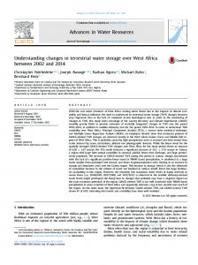
55    Haberle, et al. 2004;​ ​Denham, et al. 2003)​.  Without more thorough investigation, arguments about  population are under­determined. However, from thoroughly considering the analyses that have been  conducted, it can be determined on the basis of tool raw material type and residue analysis (​Fullagar,  et al. 2006;​ ​Summerhayes, et al. 2010)​, faunal analysis (Mountain 1991), and assemblage­level lithic  analysis (​Evans and Mountain 2005;​ ​Gaffney, Ford, et al. 2015)​ that the early inhabitants of the  highlands were very mobile people.  After the Pleistocene/Holocene transition, the focus of archaeological analysis is on the timing  of the adoption of agriculture. Figure 2­16 shows a comparative summary of models of transition to  agriculture in the highlands.   

   

56   

  Figure 2­16: Comparative models of timing of settled agriculture. Watson & Cole phases in purple; Christensen phases in  yellow; Bulmer phases in blue; Golson, Hughes and Yen phases in red; Gorecki phases in green. From Bayliss­Smith p. 502 in  Harris (ed) 1996. The gray boxes on the far right serve as a generic key linking color intensity to the subsistence practices 

   

57    described by the original authors. Lightest color intensities are wild plant food procurement (only); darkest color intensities  are the cultivation of domestic crops. Not all models contain intermediate stages. 

Current with the era in which these analyses were conducted, typology of stone tools is a heavily  utilized method (e.g. ​Bulmer 1966;​ ​Bulmer 1975;​ ​Watson and Cole 1977;​ ​White 1972)​. Working off  ethnographic studies (e.g. ​Watson 1995;​ ​White 1968;​ ​White and Thomas 1972)​ there is general  agreement that the highlanders generally used an expedient bipolar technology. Consequently an  approach of analyzing each worked edge as a type on an object was employed (e.g. ​Watson and Cole  1977;​ ​White 1972)​, although this approach still fell victim to the many limitations of applying typology  to an expedient assemblage (e.g. ​Bradbury and Carr 2012;​ ​Hiscock 2015;​ ​Shott 1989,​ ​1999)​.    All of the approaches in fig. 2­16, and Denham’s research significantly extending Golson’s  work at Kuk Swamp (e.g. ​Denham and Haberle 2008;​ ​Denham and Ballard 2003;​ ​Denham, Golson, et  al. 2004;​ ​Denham, Haberle, et al. 2004;​ ​Denham, et al. 2003)​ employ a gradual and often an  evolutionist framework. The explanations are usually centered on a pull explanation: that settling  down and adopting a sedentary lifestyle has obvious inherent benefits that people slowly  incorporated into their subsistence patterns.   Against these prevailing models, NFX is occupied from the LGM to the Pleistocene/Holocene  boundary, and pre­dates even the earliest signals of agriculture. As a group, the NFX, NBZ and NFB  sites represent a virtually continuous record from the LGM to the 18th ​ ​ century. Both NFX and NFB bear  the hallmarks of being residential occupation sites, whereas NBZ as a rockshelter is a logistical site,  and possibly also a ritual site when the rock paintings are taken into consideration. NFX provides a  benchmark for what a residential site in the terminal Pleistocene pre­agriculture looks like, against  which the assemblages of NBZ and NFB can be compared.      

   

 

58   

CHAPTER 3. PALEOCLIMATE OF NEW GUINEA  Intro:   The island of New Guinea is located a few degrees south of the equator on the Sunda shelf  separated from Australia by the shallow Torres Strait at the closest point, the Coral Sea to the  southeast, and the Arafura Sea to the southwest. The average temperature is 10°­15°C (50°­60°F) with  cloud cover, and temperatures that range up to above 33°C (90°F) in the open sun. Temperatures dip  down to 5°­9°C (40°s F) with frosts sometimes occurring especially in El Niño years where  temperatures have been recorded as low as ­2.3°C (29°F) (​Allen 2000;​ ​Pataki­Schweizer 1980;​ ​Pataki  1965)​. The high altitude forested regions receive 5­10m of rainfall in a year, while the lowland areas  only receive 2­3m of precipitation annually (​Brunskill 2004)​. While they are humid year­round, the  eastern highlands have a seasonal gradient, with rainfall heaviest in December­March, while  May­October is the dry season (​Tachikawa, et al. 2011)​. Seasonality of rain is largely controlled by the  Intertropical Convergence Zone (ITCZ) with inter­annual variability driven by El Niño Southern  Oscillation (ENSO) events (​Aldrian and Dwi Susanto 2003;​ ​Russell, et al. 2014;​ ​Tachikawa, et al. 2011)​.   These two inter­related climate phenomena – the ITCZ and the ENSO – are the controlling factors for  climate for the highlands both currently and for time periods relevant for understanding landscape  opportunities for past populations represented by the archaeological record (​Aldrian and Dwi Susanto  2003;​ ​Liu, et al. 2014;​ ​Russell, et al. 2014;​ ​Tachikawa, et al. 2011)​.   

Intertropical Convergence Zone (ITCZ)  The ITCZ is a global climate feature that roughly circles the equator. Sometimes colloquially  known as the “doldrums”, it is formed as an effect of the planet’s rotation which in turn drives the 

   

59    dominant wind directions for different latitudinal zones. Specifically, the ITCZ is formed when the  southwesterly­traveling northern hemisphere trade winds and northwesterly­traveling southern  hemisphere trade winds converge at the equator (fig. 3­1).  

  Figure 3­1: global wind patterns including trade winds converging and the ITCZ (​Kaidor 2013) 

  Observational data has demonstrated a seasonal north­south shifting of the ITCZ, with the ITCZ  moving towards the hemisphere currently experiencing summer (fig 3­2). This gradient is exaggerated  by the unequal distribution of continental landmasses and the higher albedo of the northern  hemisphere continents relative to the southern hemisphere oceans (​Böll, et al. 2014;​ ​Broccoli, et al.  2006;​ ​Philander, et al. 1996)​.   

   

60   

  Figure 3­2: global map showing idealized seasonal tracks of the ITCZ (​Halldin 2006) 

  The intensity of the Asian­Australian winter monsoon and the latitudinal location of the ITCZ  determines the quantity of wet­season precipitation in the Indo­Pacific region including the eastern  highlands of Papua New Guinea (​Leduc, et al. 2009;​ ​Russell, et al. 2014;​ ​Tachikawa, et al. 2011;  Yancheva, et al. 2007)​. The inversely­correlated variability in the Indian summer monsoon and the  Asian­Australian winter monsoon is linked with north­south variability in the ITCZ (​Böll, et al. 2014;  Böll, et al. 2015;​ ​Gupta, et al. 2003;​ ​Tachikawa, et al. 2011;​ ​Yancheva, et al. 2007)​. The ITCZ has shifted  southward over the Holocene due to increases in austral summer insolation and consequent  decreases in northern hemisphere summer insolation as a consequence of eccentricities in the  position of the Earth relative to the Sun known as the Milankovitch cycle (​Gupta, et al. 2003;​ ​Haug, et  al. 2001;​ ​Leduc, et al. 2009;​ ​Tachikawa, et al. 2011;​ ​Wang, et al. 1999;​ ​Wanner, et al. 2011)​.  Southward movement of the ITCZ has also been correlated with North Atlantic cold events such as  Heinrich events (​Böll, et al. 2015;​ ​Goswami, et al. 2006;​ ​Leduc, et al. 2009;​ ​Russell, et al. 2014)​, and 

   

61    with Northern hemisphere glaciation events(​Broccoli, et al. 2006;​ ​Russell, et al. 2014;​ ​Wanner, et al.  2011)​.  It is also notable that the ITCZ shifts southward during El Niño events (​Haug, et al. 2001)​.   

El Niño Southern Oscillation (ENSO)  ENSO refers to the variability in sea surface temperatures (SST) and atmospheric patterns in  air pressure in the tropical Pacific Ocean region. El Niño events and La Niña events are a suite of  climatological phenomena including changes in precipitation and atmospheric temperature  throughout the Pacific Basin that often accompany extreme values in the SST variability. El Niño  events are especially important to the highlands of Papua New Guinea, as they often cause extreme  droughts in the highlands and in the general Western Pacific Warm Pool (WPWP also known as the  Indo­Pacific Warm Pool or IPWP) area and the Indo­Pacific writ large. In the PNG highlands El Niño  events are frequently implicated in anomalously cold temperatures that can drop below freezing  causing destructive frosts. Droughts and frosts have caused crop failures in the highlands and  destruction of wild food sources, with serious public health consequences for modern populations  (​Allen 2000;​ ​Bourke 2000;​ ​Haberle 2000;​ ​Nicholls 2000)​. Droughts from modern El Niño events have  also created the conditions for extensive forest fires in the highlands, with attendant destruction of  property, gardens, and ecosystem (​Haberle 2000)​; and have been implicated in lowered success in  hunting wild foods (​Bourke 2000)​. With the devastating consequences El Niño events have had on  modern populations, understanding the variability in strength and frequency of the ENSO cycle is  critical for understanding changing landscape opportunities for past populations of the PNG  highlands.  

   

62    Under normal conditions, warm water accumulates on the western side of the Pacific Ocean,  especially in the region of the north coast of New Guinea and the greater area. This is called the  Western Pacific Warm Pool (WPWP) or Indo­Pacific Warm Pool (IPWP) (see fig.3­3).  

  Figure 3­3: Western Pacific Warm Pool (WPWP). Orange area around ISEA are the warmest SST. (​NASA 2016) 

  In El Niño years, the warm pool stretches east across the Pacific basin towards the equatorial regions  of South America. The atmosphere generally has low pressure over warm water due to evaporation  and convection, and high pressure over colder water. In normal years, the warm water, the low  pressure and the atmospheric moisture stays in the western Pacific resulting in the austral summer  wet season in the highlands of PNG and the general region. In El Niño years, as the warm water moves  eastward, the low atmospheric pressure and the precipitation travel with it, resulting in extreme wet  conditions in parts of the west coast of the Americas, and droughts and exceptionally cold weather in  the WPWP region generally and the highlands of PNG specifically (see fig. 3­3, 3­4).   

   

63   

  Figure 3­4: Illustration of normal vs. El Nino conditions with the migration of the warm pool eastward and attendant  precipitation patterns (​TAO_Project_Office 2016) 

 

   

64   

  Figure 3­5: Precipitation anomalies (mm) associated with moderate­strong El Niño events from 1900 to 1998. Dark areas  have precipitation deficits, hatched areas have increased precipitation. Triangles and circles represent terrestrial and oceanic  paleoclimate records respectively. (​Gagan, et al. 2004) 

  ENSO has been a major global climatic feature (fig. 3­4, 3­5) for hundreds of thousands of  years (​Tachikawa, et al. 2011;​ ​Tudhope, et al. 2001)​. However, due to the limited time depth of  various paleoclimate proxies, and uncertainty about the impact of lowered sea level and consequent  exposure of the Sunda and Sahul continental shelves on Pacific circulation, ENSO research tends to  focus on the period from the Last Glacial Maximum forward (e.g. ​Carré, et al. 2014;​ ​Gagan, et al. 2004;  Liu, et al. 2014)​.   Variations in sea surface temperatures (SST) as recorded in the differential update of  strontium and other isotopic analyses of banded corals (e.g. ​Deng, et al. 2009;​ ​Wei, et al. 2007)​ or as  recorded in the alkenone unsaturation and isotopic concentrations of foraminifera in marine  sediments (​e.g. Schwab and Sachs 2009)​. These have been some lines of inquiry into the frequency 

   

65    and amplitude of ENSO events. Varved sediments from the eastern Pacific have also been used to  interrogate the ENSO record (e.g. ​Haug, et al. 2001;​ ​Moy, et al. 2002)​, as well as the isotopic  composition of fossil bivalves from Peru (​e.g. Carré, et al. 2014)​. Recently isotopic analysis of marine  sediments from the WPWP area has been applied to the issue of understanding ENSO (​e.g. Tachikawa,  et al. 2011)​. There have been many analyses that aggregate several proxies and (e.g. ​Donders, et al.  2008;​ ​Gagan, et al. 2004;​ ​Liu, et al. 2014;​ ​Tudhope, et al. 2001;​ ​Wanner, et al. 2011)​. While this list is  not all­encompassing of the methods and results for investigating the ENSO pattern and associated  changes in SST, salinity, and direct measures of precipitation in various parts of the ENSO range, it  provides a broad foundation of data and analyses to employ in understanding the archaeological  record of places such as the highlands of New Guinea that are substantially impacted by these climate  phenomena.   

Precipitation:  In that precipitation in the highlands of PNG is affected by the latitudinal position of the ITCZ  and by the frequency and amplitude of ENSO events – phenomena that are inter­related but that are  not synonymous – it is particularly useful that some direct measurements of precipitation in the  WPWP have recently been developed. Tachikawa et al. (​2011)​ use x­ray fluorescence (XRF) of marine  sediment cores to identify variable abundances of iron (Fe), titanium (Ti), potassium (K), silicon (Si),  and calcium (Ca) in tandem with mass spectrometric analysis of the marine cores to understand the  changing sediment loads from the Sepik­Ramu river system from island  New Guinea through a  400kya time span. Ti is an especially useful indicator for coarse, refractory and heavy minerals that are  a constituent of river sediments. The marine sediment cores were collected from the Bismarck  seafloor from two locations somewhat north and west of the Sepik­Ramu basin outlet. While the 

   

66    Tachikawa et al. (​2011)​ analysis was specifically focused on understanding the role of precession and  obliquity in the hydrological processes of the WPWP over a 400ky time span, their results reveal  patterns in sediment outwash from the Sepik­Ramu basin that are relevant to understanding  precipitation from highlands that sit at the Ramu River headwaters. While the dataset that would  provide precise chronology has not yet been published, general trends are identifiable from existing  publications. Marine isotope stage (MIS) 4 (71­57kya) shows an increased contribution of coarse river  sediments. MIS 3 (57­29kya) is extremely variable with a substantial drop in sediments early in the  stage, and increasing through time. MIS 2 (29­14kya) demonstrates a substantial drop through the  stage and continues into MIS 1 (14kya­present), increasing sometime in the Holocene.  Another analysis of the coarse refractory sediment products of outwash is the Russell et al.  (​2014)​ analysis of sediments from Lake Towuti on Sulawesi. While there is some geographic distance  between the New Guinea highlands and Sulawesi (approximately 2732km straight line distance from  Kainantu, PNG to Lake Towuti on Sulawesi), these two regions experience similar seasonal  precipitation regimes, with the bulk of their rainfall occurring from November through March (​Aldrian  and Dwi Susanto 2003;​ ​Russell, et al. 2014)​.  

   

67   

  Figure 3­6: A comparison of proxy data from Lake Towuti to paleoclimate records from nearby regions. Vertical gray bars  indicate the timing of Heinrich events 1–6 (​from Russell, et al. 2014)​.  

  Lake Towuti data is presented in figure 3­6. Ti content is very low at the beginning of the  record during Heinrich event 6 (H6) at approximately 60kya, indicating reduced precipitation and  minimal river sediment contribution. There is a steep increase then a general trend downwards with  no change in sedimentation during H5 (45kya). There are peaks in sedimentation directly before both  H4 (38kya) and H3 (31kya) with an overall downward trend through this period. There is a period of  variable but overall reduced precipitation between H3 and H1 (16.8kya) with no real change in  behavior at H2 (24kya). This trend in reduced precipitation matches the drop in precipitation from the  Tachikawa et al. (​2011)​ record during MIS2. The Russell et al. (​2014)​ record shows a steep increase in  precipitation directly following the Last Glacial Maximum (24­19kya, not represented on this graph) so 

   

68    that the dry period extends from ~33­16kya, followed by a steep decrease in precipitation going to  the beginning of the Holocene (11.7kya, not represented on this graph). This pattern also has good  agreement with the Tachikawa et al. record (​2011)​ which shows a final dip in precipitation in the  Holocene with an increase towards the mid and late Holocene.   It is also notable that these patterns in precipitation have good agreement with many ENSO,  ITCZ and monsoon proxies. Liu et al. (​2014)​ note a weakening of ENSO events in the Bølling­Allerød  interstadial (BA) (~14.5kya) and an increase in ENSO events in the Younger Dryas (YD) (~12.9­11.7kya).  Donders et al. (​2008)​ find reduced ENSO activity 6­5kya, substantially increased El Niño events from  4.5­3.5kya, with a decrease towards modern ENSO activity from 3.5kya forward. Carré et al. (​2014)  note several cold events in coastal Peru 6.7­7.5kya indicating ENSO activity, and the establishment of  modern ENSO behavior at approximately 3­4.5kya. Significant El Niño activity is recorded at Laguna  Pallcachoa in southern Ecuador at 7kya (​Moy, et al. 2002)​. Extremely wet conditions linked to ENSO in  the Cairiaco Basin on the west coast of the Americas are observed from 10.5­5.4kya (​Haug, et al.  2001)​.  SST records from the Arabian Sea also support a southward movement of the ITCZ through the  Holocene linked to increased insolation, and correlated with increased ENSO activity from 2.4kya  forward (​Böll, et al. 2014;​ ​Böll, et al. 2015)​. Soil analysis from NBZ (Kafiavana) demonstrates a dry  period during the main occupation phase of 10­5kya based on the chemical composition and particle  size of aeolian deposits (​White 1972: Appendix A)   

Pollen:  There have been several pollen cores of varying timespans collected from the New Guinea  highland swamps (e.g. ​Haberle 1996,​ ​1998;​ ​Sniderman, et al. 2009)​. The longest and most complete  pollen core comes from Haeapugua in the Tari Basin of Papua New Guinea (located close to the 

   

69    marker for the Central Cordillera in fig. 2­3) (​Haberle 2007)​. While the Tari Basin is relatively more  central than the eastern highlands, this paleoecological record still offers significant insight into past  precipitation regimes.     Table 3­1: Description of pollen zones from Haeapugua in the Tari Basin, PNG. Key indicators of swamp forest biodiversity  are Myrtaceae, ​Dacrydium,​ Pandanus. From Haberle 2007 p. 223.  

  In the original article on the Tari basin, Haberle employs 19 radiocarbon dates and two know  tephra events to define the timescale of the Haeapugua Basin palynological record, with 13 of the 14 ​ ​C  dates and both tephra dates coming directly from the core that was analyzed for pollen (​1998)​. The  Tari Basin drains to the Tagali River, which ultimately drains out to the south coast (as opposed to the  Sepik­Ramu system on the north coast), and it is located approximately 350km west and slightly north     

70    of Kainantu and the Norikori Swamp. The actual precipitation measured in the heavy fraction of  sediment for the Tagali River system is not part of this analysis, and the central highlands where the  Tari Basin has a different precipitation regime than the eastern highlands that is generally wetter  more even throughout the year. However, Haberle synthesizes data from the Tari Basin with  palynological analyses from basins around New Guinea including the Norikori Swamp in defining the  ecological successions (​2007)​. The Tari Basin is one location, but the data that inform the sequence is  comprehensive across the highlands and is supported by a substantial number of dates are in good  stratigraphic order. It could be argued that ecological transitions may not happen at the same time  across the highlands, especially where anthropogenic burning is a major driver of plant regime  change, but the comprehensive nature of Haberle’s work and the strong stratigraphic control make  the Haeapugua sequence the best available measure of ecological change for the New Guinea  highlands.    The Haeapugua record (table 3­1) doesn’t start until a few thousand years into the dry period  from the Lake Towuti precipitation record with zone H3 (​Haberle 2007;​ ​Russell, et al. 2014)​.  Nothofagus, also known as the southern beech, inhabits the valley floors. Trees being long­lived  species (as opposed to herbaceous species or grasses) are more tolerant of precipitation variability.  Also the valley floors would have more moisture relative to the slopes of the valleys. Zone H4 begins  at the end of the LGM with a high fire incidence. This would be consistent with droughts and generally  dry conditions as indicated by the precipitation records and the observed incidence of wildfires during  modern El Niño­associated droughts (​Haberle 2000;​ ​Russell, et al. 2014;​ ​Tachikawa, et al. 2011)​.  During H4 there is a shift towards mixed montane forest taxa. This would be consistent with increased  precipitation and reduced El Niño activity during the BA reducing constraints on species diversity (​Liu,  et al. 2014)​. The emergence of zone H5 corresponds with the dry period associated the early  Holocene Warm Period and El Niño activity. The pollen community in zone H5 changes at ~3kya,     

71    which corresponds with the establishment of modern El Niño behavior (​Carré, et al. 2014;​ ​Donders, et  al. 2008;​ ​Haberle 2007)​.     

Summary:  Altogether, the precipitation patterns for the highlands of New Guinea as inferred or observed  from a number of lines of evidence show that this landscape experiences generally abundant but  highly variable including occasionally catastrophically low rates of rainfall. Droughts present problems  for people that range from adequate drinking water supply, water for processing resources like sago,  and complications to hunting wild game. Additionally droughts are often accompanied by frosts that  kill useful plants, both domesticated and wild. The time from first human occupation of the highland  landscape at approximately 47kya to 33kya was a period of highly variable precipitation (​Russell, et al.  2014;​ ​Summerhayes, et al. 2010)​. Drier conditions began at 33kya and continued through the Last  Glacial Maximum, after which there was an amelioration, followed by another dry period during the  early Holocene Warm Period, ending in the mid­Holocene with a return to highly variable ENSO  activity, with variability reduced at around 3.5­2kya. Changes in plant ecology as recorded in the  pollen record of the highlands of New Guinea demonstrate changes in species frequency that  chronologically correlate with changes in precipitation and El Niño activity from several proxies.     

   

   

 

72   

CHAPTER 4. DATING  Intro:   In the course of this research, two major issues regarding radiocarbon dating chronology of the  archaeological record of highland Papua New Guinea needed to be resolved. The first question  regards the date of oldest occupation of NFX. The other question regards the position of NFX, NBZ,  and NFB in the overall distribution of sites and radiocarbon dates linked with occupations throughout  the archaeological record of the PNG highlands. The first of these issues was resolved by the  identification of appropriate datable material from a unit adjacent to the unit that provided the  18,050 ±750 uncalBP date originally published in Watson & Cole (p. 194; 1977). The latter of these  issues was addressed by aggregating a database of all published radiocarbon dates associated with  archaeological materials for the highlands of PNG and analyzing patterns of site type and other site  attributes. 

   

73   

New radiocarbon date for NFX: 

  Figure 4­1: Artifact # 147, sample of wood post used for RL 370 radiocarbon date 18,050 ± 750 uncalBP plate: Tai 20 Code B  Roll 1/5 (​Burke Museum Archives 1979)  

  In the original Watson & Cole monograph, a date of 18,050 ± 750 uncalBP is published for a  “sample of mineralized charcoal post.” See fig. 2­17 for a picture of the post in situ during excavation.  Due to what was at the time surprising antiquity of age, Watson expressed significant concerns to the  contracted dating researchers about the validity of this date as well as other dates (e.g. UW 260 and  261) (​Burke Museum Archives 1979)​. At the time these samples were dated, the state of the art of  radiocarbon dating had switched from a solid­state ionization counting system originally developed by  Libby, to a gas­based system (​Taylor and Bar­Yosef 2014:290)​. Radiocarbon dating at the time was not  a particularly well­understood process by most archaeologists, and two major complications were the  need for large samples of organic material (10­12g) which were hard to find in archaeological 

   

74    contexts, and the establishment of the need for a calibration curve based on differential  concentrations of radiocarbon in the environment in the past (​Taylor and Bar­Yosef 2014)​. Watson  expressed concerns in correspondence to various researchers about changes in the water table  potentially bringing older carbon up into the archaeological sites in question or other issues of  contamination (​e.g. July 11, 1973 letter from Wastson to J. Buckley at Teledyne Isotopes, Burke  Museum Archives 1979)​. Corresponding researchers explained any relevant pre­treatment processes  (e.g. the removal of carbonate), and the unlikelihood of a sample appearing older than an accurate  date (​e.g. Aug. 5, 1974 letter to Watson from C. Tucek of Radiocarbon, LTD.; Burke Museum Archives  1979;​ ​also see Tucek 1971 for description of sample pre­treatment and dating methods)​.  None­the­less, Watson’s conservative approach towards what would have been surprisingly old dates  at the time of publication is reflected in the cautionary comments made about several dates including  RL 370 (18,050 ± 750 uncalBP) in the discussion of radiocarbon dates in the Watson & Cole  monograph (​1977:193­195)​. No geoarchaeological evidence is provided to support disturbance, and  extensive dating that would have been able to identify disturbed contexts was not available at the  time of the original research. The equivocal and conservative approach to these dates by the original  authors has created ambiguity about the validity of these dates in the larger archaeological  community, and re­dating of this site is necessary to clarify the oldest habitation of this site.  In order to validate or correct the oldest occupation at NFX, a significant portion of organic  material was identified from the unit adjacent to the unit which provided the material for the original  LGM from a level underlying the level that contains post hole fill and the artifact numbered #147  which rendered RL 370 (18,050 ± 750 uncalBP) (​Burke Museum Archives 1979)​.  

   

75   

  Figure 4­2: charcoal samples from NFX sample OxA­26323 17065 +/­ 80bp 

  Cole describes the level below the postholes in 3N14W as containing significant charcoal scatter and  numerous lithic artifacts in the NE portion of the unit (​NFX 3N14W fieldnotes, Burke Museum  Archives 1979)​. It is this material that was dated to clarify the validity of the ~18kya date from the  1977 publication (see fig. 4­2 for dated material) (​Watson and Cole 1977)​. 

   

76   

  Figure 4­3: calibration of OxA­26323 using OxCal. The red distribution indicates the uncalibrated date; the grey distribution  indicates the calibrated date with a 2σ bar; blue indicates the calibration curve (using IntCal 2009) (​Reimer, et al. 2011)​. 

  The sample sent in for dating was charcoal from a scatter from the adjacent unit to the ~18kya  date. Species of tree was unidentified. The charcoal scatter was collected from the level below the  post holes. It was associated with a small scatter of chert flakes. The new date should be considered a  terminus post quem date for the postholes and is the earliest date for human activity at the site. The  entire contents of the sample was submitted to maximize the likelihood of a result (​see Bronk  Ramsey, Higham, Bowles, et al. 2007 for pretreatment methods)​. The sample was dated using AMS  (see ​Bronk Ramsey, Higham and Leach 2007;​ ​Bronk Ramsey, et al. 2002 for AMS methods)​. The  radiocarbon sample derived from the contents of TAI20/7f was designated sample number 

   

77    OxA­26323 and returned an uncalibrated radiocarbon date of 17,065 ± 80 years before present using  the 5568 half­life (see fig. 4­3).    Using the OxCal calibration tool (​Bronk Ramsey 2010a)​ and the IntCal 2009 (​Reimer, et al.  2011)​ calibration curve, the new OxA­26323 provides a calibrated date of 20,471­20,701calendar  years ago. This date falls within the range calibrated date for RL­370 (18,050 ± 750 uncalBP) of  20,067­23,713 calBP (see fig. 4­4). As the ~18kya date has a large margin of error, and the new ~17kya  date, with a significantly smaller error margin due to improved dating methods. As both samples are  from the basal archaeological levels of adjacent units, and of similar depth, the new date of ~20kya cal  BP is a more accurate date for the earliest occupation of NFX. 

  Figure 4­4: Calibrated comparison of original date of 18,050bp to new date of 17065bp (​Reimer, et al. 2011)​. 

   

78     

Analysis of published dates from archaeological sites:  In order to understand the role of the sites excavated by Cole in relation to patterns of site use  throughout the archaeological record of highland PNG, I aggregated a database of all published  radiocarbon dates associated with archaeological material. In the case where there were  discrepancies between aragonite and collagen dates for faunal material, the date asserted by the  original author to be the more accurate was the date added to the database (​e.g. Mountain  1991:3.13)​. Dates that were from archaeologically sterile basal units and not associated with any  artifactual remains were not included in the database (​e.g. Mountain 1991: Appendix 1)​. Sites were  classified by a simple taxonomy of site types:   a) Open sites that contained general habitation artifacts and had features such as hearths that  indicate domestic activities. There are no indications of agricultural activities at these sites.  b) Rockshelters that were sites of either general or specialized use but that were located in small  caves.  c) Agricultural sites that were located in swampy areas and contained features that indicated  agricultural activities such as mounds, ditches, or other small earthworks relevant to  regulating moisture for plants.   All sites types contain chipped stone tools with usewear indicating several different activities and with  food residues (​e.g. Fullagar, et al. 2006)​.   This database of radiocarbon dates was analyzed using OxCal to generate uniformly calibrated  dates and a graphical representation of the dates for visual comparison with various paleoclimate  reconstructions both regional and global (see Appendix A for list of sample numbers, uncalibrated and  calibrated dates, source publications and other details) (​Bronk Ramsey 2010b)​.   

   

79   

  Figure 4­5: All radiocarbon dates from archaeological deposits from highland PNG calibrated using OxCal and the IntCal 2009  calibration curve. Bars at the top of the calibration show the time span for different site types. Blue bars on the main 

   

80    calibration graph represent major global climate cold events. The bar below the calibration graph shows the major ecological  regimes based on pollen cores from the Haeapugua Swamp (Haberle 2007).  

This visual matching of radiocarbon data with global and regional climate data suggests a  correlation between major climate events and shifts in site use with a possible gap around the  Heinrich 4 (H4) event, the beginning of continuous use of rockshelters in the LGM (with first use of  rockshelters in the H3 event), and the advent of agricultural sites at the end of the Younger Dryas.  Anthropogenic fire may drive a transition from closed canopy forest to grassland very quickly, while  large scale climate alterations from warmer to cooler, or wetter to drier affect plant species  composition more slowly. Tropical trees generally grow quickly due to the abundance of water,  although there is variability between species (​Bazzaz and Pickett 1980;​ ​Nicholas 1985)​.  The  palynological ecological reconstructions (i.e. Haeapugua pollen stages) are lagging indicators, with  global climate trends (e.g. LGM, YD, etc.) and archaeological site use change preceding the  palynological changes see figure 4­5 above). As one might expect archaeological site use change to  follow changes in ecological communities of desirable plants and animals, this was a surprising  finding, indicating that a different environmental constraint was at play with the patterning of site  use. Validating these possible relationships was a key target of the ​SPD analysis.  One important outcome of the comparison of all radiocarbon dates with global climate data is  to establish that there was indeed an LGM occupation of the PNG highlands, contra Summerhayes et  al. 2010. The dates of the LGM are defined by Clark et al. 2009 as spanning from 26.5­19kya at its  maximum in the northern hemisphere. Sites in PNG that fall within this time period include AER in the  Ivane Valley, NFX in the Kainantu Valley, JAO also known as Wañlek, and NAC or Nombe. The Clark et  al. (​2009)​ dates are generated from 4443 radiocarbon dates from samples, calibrated with CALIB ver.  5.02 for dates less than ~24kya, and dates with the Fairbanks calibration for dates older than ~24kya  (​see Clark, et al. 2009 supporting online materials for further details)​. The Fairbanks curve dates fall  within the IntCal 2005 curve for the period of time relevant to the LGM (​Fairbanks, et al. 2005;     

81    Reimer, et al. 2011)​. The IntCal 2009 curve was largely an extension of the IntCal 2004 curve that only  calibrated to ~26kya (​Reimer, et al. 2004;​ ​Reimer, et al. 2011)​. The CALIB calibration program uses the  IntCal curve for calibration. The new date provided above (fig. 4­3) from NFX ~20kya cal. falls within  the date range of the LGM, as does the previously published oldest date from NFX from the Watson  and Cole monograph ~22kya cal as well as the other dates mentioned above (​Watson and Cole 1977)​.  Haberle (​2007)​ does not comment on his calibration strategy, but Golson (​2005:231)​ notes that  several highland PNG researchers use an unpublished table developed by Haberle for calibration, and  that this table is based off of the CALIB ver. 3.1 program and presumably an early version of the IntCal  calibration curve. Without further clarifying information, it is assumed here that this is the method  used for calibrations in Haberle’s publications.   

Testing hypotheses with ​SPD  In order to test hypotheses about the relationship of changing site types and global climate  phases, the radiocarbon dates in the aforementioned database were analyzed again, this time using  summed probability distributions (​SPD) and kernel density estimates (KDE). Working with William  Brown of University of Washington, a number of analyses were produced. Statistical methods used  are described in Brown 2015, and original R code written by Brown was used to produce these  analyses. These analyses, while promising, are also provisional due to the limitations of the small  number of dates available and the demand for larger sample sizes for robust results. Robust ​SPD  preferably uses over 500 sites, whereas the available dataset had only approximately 130 dates total,  which summed to 76 actual dates used in the analysis. Because of the sample size limitations, no  demographic arguments can be made with this dataset (​see Attenbrow and Hiscock 2015 for a fuller  discussion of the limitations of ​SPD for demographic change)​. As we are not seeking to make a 

   

82    demographic argument but rather one of variability in site use, the results of this analysis have proven  to be useful in understanding patterns in changing site types through time. Earlier in the Pleistocene,  changes in proportions of site types look quite extreme, but this is an artifact of the low number of  dates in this time range and may not reflect the actual population. Proportions are more reliable in  the very terminal Pleistocene and through the Holocene as this is where the density of dates lies and  sampling error will be less of a problem. 

   

83   

  Figure 4­6: Secular variation in type­to­type proportions calculated using kernel density estimates (KDE) that have been  rescaled to subset sample size. This shows the changing proportions of site types (open sites, rockshelters, and agricultural  sites) as determined by all published radiocarbon dates for archaeological contexts for the highlands of Papua New Guinea.  Use of logistical sites (rockshelters) begins ~33kya, intensifies after the LGM. Blue bars represent global climate cold events.  Yellow and orange bars represent the onset and intensification of mid to late Holocene ENSO activity. The dates of global  climate events are supported by hundreds of radiocarbon dates from various sources, details in the supporting materials of  the articles.  

 

   

84    Through the lens of ​SPDs of specific types as a ratio of all sites of all types, patterns in  changing frequency of site types is confirmed. Looking at fig. 4­6, there is an initial use of rockshelters  in the H3 phase (at Nombe; Evans & Mountain 2005) that is not continuous, but re­emerges in the  Last Glacial Maximum when the continuous use of rockshelters begins. Open sites gain in proportion  to other site types at the end of the Younger Dryas, as agricultural sites emerge, and rockshelters lose  importance. Rockshelters have a steep decline in importance as agricultural site use increases in  intensity in the early mid­Holocene as ENSO activity kicks up, while the proportion of open domestic  sites stays relatively steady through this period. The proportions of sites (fig. 4­6) during the  Pleistocene are likely distorted by the very low number of dates in this range, but the analysis  becomes more robust in the very terminal Pleistocene and Holocene due to the increasing number of  dates (see fig 4­7 for histogram of dates, and Appendix A for radiocarbon date data set). 

  Figure 4­7: histogram of number of calibrated 14C dates used in this analysis. See Appendix A for complete details of data  set. 

   

85     

Summary:  Through the radiocarbon analysis of organic archaeological material associated with lithic  artifacts and from a similar depth in an adjacent unit, the LGM occupation of NFX is confirmed with a  date of 17,065 ±80 uncalibrated radiocarbon years, or 20,701­20,471 calibrated calendar years. This  new data point was incorporated into a database of all published radiocarbon dates associated with  archaeological materials in for the highlands of PNG. This dataset was calibrated with OxCal using the  IntCal 2009 calibration curve and compared to a number of paleoclimate datasets both regional and  global. It should be noted that additional radiocarbon dates for Wañelek have been published  (​Gaffney, Summerhayes, et al. 2015)​ since the radiocarbon date database was aggregated, but it is not  expected that these dates will significantly alter the final analysis of changing ratios of site types.  Dates from several sites in the highlands including the new NFX date fall within the established  timespan of the LGM. Additionally, this visual comparison gives rise to questions whether changing  site type use is linked to larger climatic changes as opposed to local ecology. Towards evaluating the  models presented in Chapter 1, the shifting importance of different site types and global climate  phases are explored through a provisional summed probability distribution analysis of sites by type,  and changing rates of the ratio of different site types to the whole established in relation major  climate trends. Major climate changes – especially the LGM, the Younger Dryas, and the  mid­Holocene increase in ENSO activity – is closely associated with changes in the proportion of site  types. The use of rockshelters increases from the LGM to the YD, when agricultural sites start building  in importance relative to rockshelters, while the proportion of open sites remains fairly even from the  YD forward.   

   

 

86   

CHAPTER 5. ARTIFACT ANALYSIS  Introduction:  Between 2010 and 2015, I measured, quantified, and otherwise described over 2,000  unmodified flakes, 75 amorphous cores, a handful of bifacially reduced tools, and 81 unifacially  reduced tools. I also cataloged hundreds of other non­lithic artifacts with some quantitative or  nominal data about these objects. These objects came from the assemblages of the eastern highland  Papua New Guinea archaeological sites of NBZ (Kafiavana), NFX and NFB (see fig. 5­1 for locations of  sites).  

  Figure 5­1: Map of archaeological sites in the eastern highlands. 

 

   

87    I used a flexible approach towards sampling to balance between representation of  assemblages and practical limitations on time. As the assemblage was quite large, I used a 10%  sampling of the assemblage from NBZ. I examined a total n=1,312 artifacts from NBZ, with 1,150 of  them being unmodified flakes alone. The number of artifacts in the full assemblage was not recorded,  but would fall somewhere above 10,000 artifacts. At NFX the assemblage was much smaller, so I used  a 100% sample of excavated materials (N=497, with expedient or unmodified flakes being 467 of that  assemblage). I sampled a smaller proportion of debitage bags from NFB (n=105; levels 1­8  represented), and a 100% sample of artifacts that had been identified in the Watson/ Cole analysis of  the NFB material (n=724 artifacts identified by Watson & Cole; n=829 total). Generally Watson and  Cole identified lithic artifacts with evidence of usewear visible to the naked eye or with some retouch  or other sort of secondary reduction. Watson and Cole also identified non­chipped stone artifacts  such as raw quartz crystals, ochre, animal bone, plant samples, and pottery sherds. In the statistical  analysis, I only used expedient flakes with usewear. Debitage that had not been used as a tool would  be underrepresented at NFB due to limitations of sampling of the level bags that contained artifacts  that were collected but not individually cataloged in the original Watson and Cole monograph (​1977)​.  I examined and recorded a total of 2,638 artifacts in the course of this project.   

Results from the lithic analysis:  The original data collection design for the lithic assemblage included both a general debitage  analysis strategy, and data points that were targeted at measuring intensity of reduction to be used as  a proxy for mobility of past populations. Generally, the assemblage can be described as consisting of a  large number of irregularly­shaped and relatively small flakes. There are also a number of bipolar  reduction objects that are interpreted as bipolar cores. There are significant methodological and 

   

88    theoretical complexities to understanding the role of bipolar cores, variously known as scalar pieces,  pieces esquilles, wedges, splintered pieces to name a few (e.g. ​Bradbury and Carr 2012;​ ​Hiscock 2015;  Leblanc 1992;​ ​Shott 1989,​ ​1999)​. This analysis was not designed with the intent of understanding the  role of bipolar reduction in the assemblages at hand, but rather to understand retouched pieces.  Between the theoretical and methodological complexities and the different research questions that  shaped the analysis strategy, what can be said about the bipolar reduction strategy is fairly limited.  There is also very little that can be said about the measures of reduction (GUIR and Clarkson’s index of  invasiveness) due to the uneven distribution of relevant artifacts in two of the sites (NFX and NFB).  Bipolar reduction is the dominant strategy for reduction based on the small, irregular, expedient  flakes that dominate the three assemblages considered here. Due to the ambiguity of the role of  bipolar objects in the reduction sequence as either core or tool (​Shott 1989,​ ​1999)​, and due to the  frequent presence of edge damage indicative of usewear, bipolar objects were included in the  unmodified flakes dataset as they had identifiable ventral surfaces or were otherwise identifiable as  the product of a chipped stone technology as opposed to being produced by natural processes.   Size and weight, as well as amount of cortex are used as measures of reduction to reveal if  patterns in mobility can be detected. Sites with a large variability and a higher mean in size of artifacts  are interpreted as long­term residencies, which have been provisioned with raw material, and  therefore material at all stages of reduction should be present (​Binford 1979;​ ​Kuhn 1991,​ ​1993,​ ​2004;  Nelson 1991)​. Sites with lower means and lower variances are interpreted as sites where there is a  high level of mobility, as high­quality material will be thoroughly reduced into small pieces (​Binford  1979;​ ​Kuhn 1991,​ ​1993,​ ​1994)​. Likewise, sites with more cortex are interpreted as provisioned,  long­term occupation sites where all stages of reduction occur; camp sites of highly mobile people will 

   

89    have little to no cortex as only the highest quality material will be transported in frequent moves  around the landscape (​Binford 1979;​ ​Nelson 1991)​.  Quantitative, nominal, and qualitative data about the shape and other characteristics of the  lithic assemblages of NBZ, NFX and NFB was collected into a series of Microsoft Access 2010  databases. Lithic artifacts comprised the bulk of these archaeological assemblages. Data about the  frequency of other artifact types was also collected. Data was exported to Microsoft Excel 2010  spreadsheets. Some analysis was conducted in Excel. Data was also imported into SPSS 19, and  analysis was conducted with that application as well. All datasets as well as other electronic products  such as scanned notes, digitized maps, etc., will be archived with the Burke Museum of Natural  History and Culture at the University of Washington in Seattle, WA, USA.   

Descriptive statistics on flakes with usewear:   Supplementary data regarding graphs and charts presented here can be found in Appendix B. 

Maximum length of flakes with usewear:    Table 5­1: descriptive statistics for the max length of unmodified flakes with usewear 

Max Length in mm  Descriptive Statistics 

   

 

 

 

 

 

 

 

 

   Mean  Standard Error  Median  Mode  Standard Deviation  Sample Variance  Kurtosis  Skewness  Range  Maximum 

NFX  24.6  1.3  22.8  13.1  11.0  121.8  14.8  3.0  77.7  87.6 

NBZ  20.0  0.7  18.6  14.4  8.8  78.0  1.2  1.1  43.8  51.1 

NFB  20.7  0.5  19.8  15.9  7.5  56.1  7.2  1.7  58.6  65.5 

   

90    Minimum  Sum  Count  Geometric Mean  Harmonic Mean  AAD  MAD  IQR   

10.0  1718.8  70.0  22.9  21.5  7.2  5.3  10.3 

7.3  3223.4  161.0  18.3  16.8  6.8  5.7  11.1 

6.8  5555.8  268.0  19.6  18.5  5.6  4.5  9.1 

The boxplot (see fig. 5­2) is a useful tool for visualizing the differences in sample populations.  The boxplot shows quartiles, with the transition between colors in the solid box representing the  mean of that distribution. See Appendix C for quartile transitional values for boxplot. The long upward  tail of the lengths of the expedient flakes with usewear is to be expected since there is a lower limit in  which a) people are able to use a tool, and b) that researchers will be able to collect using standard  excavation methods such as screening with hardware cloth. Moreover, stone tool production is a  reductive technology – smaller tools are made out of larger ones. This is especially true of the  expedient collections here where every object is recycled without specific constraints to shape, and  the distinction between “core” and “tool” is largely irrelevant. 

   

91   

  Figure 5­2: Sites are ordered oldest to youngest. ​14​C dates indicate NFX was occupied from ~18kya­11.5kya; NBZ from  ~10kya­5kya; NFB from ~3.8kya­185ya. This is graphical boxplot of distribution of values for maximum length in mm of flakes  with usewear. Transitional values can be found in Appendix C. 

  ANOVA, or Analysis of Variance, is a statistical strategy to compare multiple populations at the  same time instead of only a pairwise comparison. ANOVA does not analyze variance, but rather the  means of several sample sets simultaneously to determine whether or not they come from the same  population. An F test score that is substantially higher than 1 indicates that there are substantial  differences in the means of the sample sets, and they are determined to not being from the same  underlying population. A low P­value indicates that the likelihood of getting the F test score when the  null hypothesis (that the sample sets come from the same population) is extremely unlikely,  supporting the falsification of the null hypothesis. ANOVA is robust against violations of the  assumption of normal distribution, so skew (table 5­1) in this case is not a problem (​Drennan 1996;  Ramsey, et al. 2001)​. 

   

92    Table 5­2: ANOVA analysis of distributions for values of maximum length of unmodified flakes in mm with usewear. High F  value and low P value confirms that differences in means are not random. 

    As the ANOVA (table 5­2) shows us that the length of unmodified flakes with usewear from all  three sites don’t come from the same parent population, a set of T­tests are used to determine where  the difference lies. The T­test is robust to skewed distributions when the numbers are large (​Ramsey,  et al. 2001)​.  

   

93      Table 5­3: T­Test for distributions of maximum length of unmodified flakes between NFX & NFB. High t­stat and low p­values  indicate that these assemblages represent different populations.  

    As the variances (table 5­3) between NFX and NFB are fairly dissimilar (without performing an  F­test), the lower part of the table for T­TEST: Unequal Variances should be used. In both cases  (one­tail and two tail) the ​t­stat is greater than the ​t­crit, and the ​p­values are quite low (