JOURNAL OF COMPUTATIONAL BIOLOGY Volume 8, Number 4, 2001 Mary Ann Liebert, Inc. Pp. 443–461
Unfolding of Microarray Data ANDREW B. GORYACHEV,1 PASCALE F. MACGREGOR,2 and ALED M. EDWARDS2
ABSTRACT The use of DNA microarrays for the analysis of complex biological samples is becoming a mainstream part of biomedical research. One of the most commonly used methods compares the relative abundance of mRNA in two different samples by probing a single DNA microarray simultaneously. The simplicity of this concept sometimes masks the complexity of capturing and processing microarray data. On the basis of the analysis of many of our microarray experiments, we identi ed the major causes of distortion of the microarray data and the sources of noise. In this study, we provide a systematic statistical approach for extraction of true expression ratios from raw microarray data, which we describe as an unfolding process. The results of this analysis are presented in the form of a model describing the relationship between the measured uorescent intensities and the concentrations of mRNA transcripts. We developed and tested several algorithms for inference of the model parameters for the microarray data. Special emphasis is given to the statistical robustness of these algorithms, in particular resistance to outliers. We also provide methods for measurement of noise and reproducibility of the microarray experiments. Key words: cDNA microarrays, gene expression, statistical data analysis. 1. INTRODUCTION
D
NA microarrays are used to explore gene expression on a genome-wide scale (Brown and Botstein, 1999; Duggan et al., 1999). By quantifying the relative abundance of thousands of mRNA transcripts simultaneously, researchers can discover new functional relationships among genes (Wen et al., 1998) and observe the response of whole genomes to various experimental perturbations (Iyer et al., 1999; Spellman et al., 1998). Microarrays have also found extensive application in medicine and pharmacology (Debouck and Goodfellow, 1999). For example, microarrays can be used to identify genes whose pattern of expression distinguishes various types of cancer (Alizadeh et al., 2000; Golub et al., 1999). There are two major types of DNA microarray technologies that can be broadly termed as one-channel and two-channel. The one-channel measures the absolute concentrations of mRNA transcripts. The twochannel estimates the relative abundance between a sample and a control specimen. In this second method, which is the focus of this paper, uorescently-labeled cDNA is prepared from the two biological sources that are to be compared. The two cDNA populations are labeled with different uorescent dyes, pooled, and simultaneously cohybridized to thousands of different DNA molecules, which are arrayed on a modi ed
1 Ontario Cancer Institute, Princess Margaret Hospital, Toronto, Canada. 2 C. H. Best Institute, University of Toronto, Toronto, Canada.
443
444
GORYACHEV ET AL.
glass slide. The uorescence from the glass slide is measured at the two wavelengths and the individual microarray spots are identi ed using image-processing algorithms. The background uorescent intensity can then be subtracted from the intensity of each spot. Finally, the two data sets, one for each uor, are scaled to each other and the normalized intensities at each spot are compared to generate a list of genes that are differentially expressed. The success of DNA microarray analysis is critically dependent on the quality and precision of the data, but the miniaturization and massive parallelization involved pose challenging physical and mathematical problems for data acquisition and subsequent analysis (Chen et al., 1997; Claverie, 1999; Schuchhardt et al., 2000). Because gene expression levels in cells can vary by several orders of magnitude, it is necessary to measure signals over a wide dynamic range. In microarray experiments, it is common to observe both saturated signals and signals that are lost in the background noise. For low intensity spots, distinguishing the targets from the background poses signi cant challenges and inevitably results in large measurement error. The integration and scaling of the two data sets are also dif cult for two reasons. First, the two commonly used ors, Cy3 and Cy5, have different physical properties. They are differentially incorporated into the cDNA, and the quantum uorescent yields are different. Second, the microarray spots are widely separated with respect to their individual size and thus spots may be hybridized, washed, and scanned in different conditions depending on their location on the array. There are various algorithms that accomplish the target separation, background correction, and normalization steps. For the DNA microarray applications, these methods are commonly disseminated by means of web sites or through private communication. A number of recently developed software packages also provide numerous options for image quanti cation, background correction, and normalization. The dif culty in selecting the optimal suite of programs for data reduction stems from the fact that the underlying algorithms are rarely known and their relative performance is dif cult to assess. In addition, many of the methods have not been suf ciently substantiated by statistical analysis. In particular, the statistical robustness of background correction and normalization methods has not received adequate attention since the pioneering paper by Chen et al. (1997). In this paper we provide a systematic statistical approach to dealing with raw DNA microarray data. We introduce a model that describes a relationship between the measured uorescent signals and the mRNA concentrations. This model stems from the analysis of many of our microarray experiments, including several that were designed speci cally to assess contribution of factors that complicate microarray analysis. We show that one can extract true expression ratios from the raw microarray data by statistically estimating the parameters of the model. In broad terms, our technique is analogous to the method known in statistical data analysis as unfolding (Cowan, 1998), and our work presents a uni ed framework for the unfolding of microarray data.
2. MODEL FOR MEASURED EXPRESSION RATIOS The goal of this section is to introduce a model that describes the relationship between the intensities of uorescent signals and the concentrations of mRNA transcripts. To achieve this, we must account for the sequence of chemical and physical processes that take place between the RNA isolation and the quanti cation of the microarray image. In our notations, let the RNA messages for the i-th gene be present at concentrations cis and cic in the sample and control specimens, respectively. For the sake of clarity, we temporarily assume that the sample is labeled with Cy3 (“green”) and the control with Cy5 (“red”). The other labeling order is possible and often necessary to determine the systematic effects introduced by the type of or (see Section 3.3). Therefore, it is important to distinguish sample and control probes from “red” and “green” channels. If the reverse transcriptase incorporates on average °i molecules of dye into the cDNA copy of the i-th transcript, then after labeling the i-th gene is represented by °iG cis optically detectable molecules in the sample and °iR cic in the control. In practice, the ef ciency with which the dye is incorporated °iG , °iR depends on the conditions of the reverse transcription (RT) reaction, the ternary structure of mRNA, and the gene nucleotide sequence. The quantity °iG is not generally equal to °iR due to the difference in molecular properties of the dyes, and the preferential incorporation of the dyes into speci c cDNAs can be reproducibly shown in experiment.
UNFOLDING OF MICROARRAY DATA
445
After the hybridization of the labeled cDNA to the DNA on the microarray surface, the resulting uorescence is quanti ed using uorescence microscopy. The intensity IiG .r / of the green uorescent signal from the i-th gene spotted at location r on the array is proportional to °iG cis with a coef cient AG . The scaling factors AG , AR incorporate the quantum yield of dyes (i.e., ef ciency of emission) and the sensitivity of the scanner. Since the excitation and detection of uorescence are performed separately for red and green channels, the uorescent properties of dyes are different, AR and AG are not identical. In fact, they can vary widely depending on the scanner parameters (e.g., laser emission power and photomultiplier voltage). In some experimental layouts, AR and AG depend on r . This dependence can be explained in part by the spatial microheterogeneity of the hybridization conditions and also the warped shape of the glass slide. The spatial heterogeneity of AR and AG may also arise as a consequence of the optical design of the scanner if it is based on confocal microscopy. The typical focal depth of a confocal scanner is 25 ¹m. Given the dimensions (25 £ 75 mm) of a typical microarray glass slide, even in nitesimally small angles of 10¡3 in the position of the slide during scanning could result in the gradual loss of focus as the scanning beam sweeps across the array. This imperfection manifests itself in A.r / gradients observed in top–bottom and left–right directions on the array (see Section 3.2 for discussion). The description of the microarray signal intensities is complete when stochastic terms »iR .r /, »iG .r / representing all noisy contributions to Ii .r / are added. They take into account the cumulative effects of chemical, optical, and computational factors that are introduced by the microarray technology. One of the major challenges in the analysis of the microarray data stems from the fact that assessing and controlling the relative contributions of the many sources of noise is dif cult. Chemical factors, such as those introduced during RNA preparation, labeling, hybridization, and washing, contribute to the » terms in two ways. Most of the variability derives from incomplete hybridization or nonspeci c binding to the array. The nonspeci c binding appears to be more of a problem for genes with a higher content of low-complexity sequence motifs (hence subscript “i” in the »iR .r /, »iG .r / terms). The issues and complexities of correction for the background signal, whose nature is primarily de ned by the chemical factors, require special attention and are considered in a greater detail in Section 3.1. Optical noise derives from factors intrinsic to uorescence microscopy (Inoue and Spring, 1997). For example, the background current from the photomultiplier tube (PMT), the “dark current,” complicates the analysis of low-intensity spots. Computational variability arises from errors introduced by the quanti cation algorithms. For example, distinguishing the pixels in a target from those in the background is a challenging image recognition problem since the microarray spots often have low intensity and imperfect morphology. Finally, assembling all introduced terms as shown in Fig. 1, we can present the observed green/red signal ratio, Ti .r /, as Ti .r / D
IiG .r / IiR .r /
D
AG .r /°iG cis C »iG .r / AR .r /°iR cic C »iR .r /
:
(1)
This equation demonstrates that the observed value Ti .r / can be a fairly distorted representation of the actual ratio of sample and control mRNA concentration Tia D cis =cic , which is the nal goal of the microarray experiment.
3. THE MAIN STEPS OF THE UNFOLDING The model introduced in the previous section provides a theoretical framework for the unfolding of microarray data. Our model explicitly takes into account the most important factors that are thought to distort the true expression ratios Tia . For the practical analysis of microarray data, it is important to distinguish distorting factors that can be inferred from a single microarray from those factors that require multiple repetitions of the microarray experiment. The rst category is mainly constituted by factors that are independent of the gene and vary continuously with location on the array (e.g., scaling factors AG;R .r /, whose dependence on r is de ned by conditions of hybridization and distance to the scanner lens). The second category consists of factors that vary markedly with both gene and location, such as nonspeci c binding and quanti cation errors.
446
FIG. 1.
GORYACHEV ET AL.
Diagram illustrating the derivation of the model (1) for the measured ratio of uorescent intensities.
Before going into the detailed discussion of individual steps, we give an overview of the entire unfolding procedure and stipulate the limits of the unfolding set forth by the noise factors. From the form of the model (1), it follows that one should remove the additive terms »iR;G .r / as the rst step towards extracting Tia from the experimental value Ti .r /. However, it is generally impossible to nd exact estimates for the »iR .r /, »iG .r / terms for each spot due to the stochastic nature of factors contributing to the noise terms. A closer look at the raw microarray data shows that the »iR;G .r / terms possess a signi cant systematic component from the background uorescence. For example, in Fig. 2A, we show that additive background terms can profoundly affect the measured ratios. As the signal intensity diminishes, one observes deviation of the expression data from the straight line, which re ects the growing in uence of the »iG .r / terms. At low intensities, the numerator of (1) is dominated by »iG .r /, whose average value saturates while the denominator diminishes. We can calculate an estimate for the systematic components of the background signal, e.g., the most probable values per channel, B R .r /, B G .r /, from the raw data. The “truly random” zero-centered noise can be obtained by subtracting the systematic components B R .r /, B G .r / from the terms » R .r /, » G .r /.
FIG. 2. Unfolding of the microarray data. (A) Generic raw data, tted to the data equation I G D a C bI R , is shown by the solid line. (B) Same data after correction for the background and normalization.
UNFOLDING OF MICROARRAY DATA
447
This residual noise contributes to the scatter of the expression points but does not lead to their systematic deviation from a straight line. We now can rewrite model (1) in the form Ti .r / D
AG .r /°iG cis .1 C "iG / AR .r /°iR cci .1 C "iR /
;
where the noise terms are moved inside the product. Here we assume that the statistical properties of the residual noise do not depend on location on the microarray. Since "iG , "iR are purely stochastic, their contribution cannot be ltered out. Therefore, as the result of the unfolding of a single microarray, we nd the effective expression ratios Tie , which are equal to cQis =cQic , cQi D ci .1 D "i /. By simplifying the previous equation further, we nally get Ti .r / D
AG .r /°iG AR .r /°iR
¢ Tie :
After background correction, the entire set of expression data is stretched on the plane (I G , I R ) along a certain line which is parallel to the main diagonal and offset by the ratio of scale factors AG .r / and AR .r /. We can remove systematic distortion of expression ratios due to the scale factors AG .r /, AR .r / and center the data points around the line I0R D I0G (Fig. 2B) by applying one of the normalization methods described below. The last step of the unfolding is the correction for the differential dye incorporation represented by the °iG , °iR terms. Since incorporation coef cients do not depend on the location and vary widely from gene to gene, they cannot be inferred from a a single microarray experiment. A special experimental procedure involving the two possible variants of labeling and known as “dye switch” or “dye ip” is required to provide the data necessary to estimate the incorporation coef cients. Finally, the unfolding transformation, which allows us to calculate effective expression ratios Tie as the best approximation for the actual ratio Tia , can be symbolically written as Tie D
°iR AR .r /.IiG .r / ¡ B G .r // °iG AG .r /.IiR .r / ¡ B R .r //
:
(2)
In practice, the transformation (2) is calculated using the numeric algorithms presented in the following subsections. Our method accounts for a number of practical problems associated with background correction, normalization, and correction for the differential labeling. We describe these problems in the following sections.
3.1. Background correction The treatment of background is possibly one of the most controversial and the least explored problems of microarray data analysis. Before discussing strategies for background correction, it is important to de ne how the target and the background signals are determined in the course of the image quanti cation. In this study, we assume that the quanti cation software performs image segmentation (i.e., separation of different targets) and integrates all pixels covered by a mask of regular shape and constant size. The size of the mask is chosen suf ciently large to encompass the entire spot and possibly some of the surrounding area. The intensity of the target is then de ned as the integral pixel count averaged over the mask. The intensity of the local background is calculated in the area surrounding the target mask so that target masks of the neighboring spots are excluded. This quanti cation method ensures that pixels belonging to the spots are not attributed to the background and the background level is not overestimated. Many image quanti cation packages provide an option to automatically subtract the local estimate of the background from the intensity of the corresponding spot. This method of background correction is not generally recommended, for two reasons. Firstly, typical background signal demonstrates signi cant variation with location on the array. Local background estimates may be affected by small-scale uctuations with high amplitude and their subtraction might result in additional noise in calculated expression ratios.
448
GORYACHEV ET AL.
Secondly, substantial systematic error can be incurred in regions of the microarray which are obviously defective and characterized by unusually high level of background (e.g., regions with uorescent smears). In such regions, it is not uncommon to observe spots that have intensities lower than the surrounding background. It is clearly inappropriate to subtract the background in such areas. Instead, they must be identi ed and processed separately from the rest of the array. Thus, the treatment of background can be split conceptually into two problems: to locate areas of the microarray occupied by defects with abnormal background properties and to nd the optimal estimates for the background correction factors B R .r /, B G .r / for spots which are not affected by defects. The defects, which commonly result from slide coating failures, chemical stains, smudged spots, and dust particles, are easily detectable by a human eye. However, identi cation of defects presents a signi cant challenge for image quanti cation software and is not even attempted by many programs. We developed statistical means to separate regions of homogeneous background from those that harbor signi cant defects. Our method is based on the properties of the probability density function for the local background counts on the microarray. Figure 3A shows probability density functions for the logarithm of background intensity (PDFL) calculated for three typical background samples (see Section 5.2 for sample de nition). The logarithmic transformation (see Section 5.1) was used to facilitate subsequent application of numeric algorithms relying on quasi-symmetry and quasi-normality as the original probability density functions (PDF) for the intensities were found strongly asymmetric and skewed to the right. The three samples represent three consecutive degrees of contamination by the defects. Case a is an “ideal” background without inhomogeneities and defects, while c contains signi cant defects, such as extended bright blotches. The presence of the defects can be inferred from the form of the right tail of the respective PDFLs. Thus, in case a, the PDFL vanishes faster than that for b. In case c, the defects are so prominent that they form a second maximum at very high intensities. Further insight into the statistical properties of the background can be gleaned from the normal quantile–quantile plots, which are shown for the same three background samples in Fig. 3B. Remarkably, the PDFL for the normal homogeneous background (a) shows only minor deviation from the normality. Samples b and c clearly demonstrate an earlier departure from the normality, which can be attributed to the presence of the defects. Therefore, we assume that the “ideal” background is described by a normal PDFL (log-normal PDF) with possibly slightly different standard normal deviations for the right (¾ C ) and left (¾ ¡ ) tails. These observations can be employed to resolve areas with homogeneous normal background from G R defective areas. The aim is to seek an upper estimate for con dence limits I B , I B such that if the local background intensity exceeds it, then, with a certain con dence (e.g., 95%), the corresponding area is G R deemed defective. To nd upper con dence levels I B , I B , one needs to estimate the parameters (¹, ¾ C ) for the right-side normal t of the respective empirical PDFLs. Since experimental PDFLs are approximated
FIG. 3. Statistical properties of the background. (A) Probability density functions for the logarithm of the background intensity (base 10). (B) Normal quantile–quantile plots for the PDFLs shown on the left panel.
UNFOLDING OF MICROARRAY DATA
449
by a normal function only near their mode, it is important to use robust methods to estimate the parameters. Thus, we found the least trimmed squares (LTS) estimator mLT S (Rousseeuw and Leroy, 1987) useful for calculation of the mode ¹. In the LTS method, the squared regression residuals are computed as in the usual least squares method. However, only a fraction ® of the smallest residuals is retained and used for minimization. In this treatment, mLT S is resistant to the presence of up to .1 ¡ ®/ ¢ 100% of outliers. Given robust estimates for the parameters (¹, ¾ C ) and applying the “rule of two sigma” which gives 95% con dence for a normal distribution (Snedecor and Cochran, 1973), for the upper con dence limit I B we nally get I B D exp.¹ C 2¾ C /: After setting aside the defective areas, the background correction factors B G;R .r / are calculated for the spots in regions of homogeneous background. We argued above that the local background found by the image quanti cation software can exhibit undesirably high variability due to the abrupt spatial uctuations in background intensity. To avoid this problem one can calculate B G;R .r / as the median background intensity computed for some neighborhood centered at r with size ±. The larger the ±, the higher is the con dence that B G;R .r / will not be affected by the outliers. At the same time, the choice of excessively large ± can result in the loss of important information on the spatial variation of the background. Therefore, it is necessary to nd the optimal size of the sampling neighborhood so that B G;R .r / is both outlier resistant and suf ciently sensitive. To achieve this, we investigated the spatial correlation of the background using Fourier analysis (see Section 5.2). Figure 4 shows typical Fourier power spectra in which the ordinate value Pk represents the contribution of the spatial frequency k=L (k D 0; : : : L=2; L D 200). The sharp maxima at low k indicate the presence of signi cant long-range background gradients. For k > k ¤ ¼ 20, the spectrum is essentially at and the equal contributions of high frequencies create noise on top of the long-range spatial modes. Therefore, it is reasonable to accept ± D L=k ¤ as the optimal size of the sampling neighborhood . For the example shown in Fig. 4, we nd that ± approximately corresponds to six distances between spots. Thus, neighborhood s of 5 £ 5 or 7 £ 7 spots are optimal for the background sampling.
3.2. Normalizatio n In practice, the scale factors AG .r / and AR .r / described by our model cannot be directly extracted from the experimental data. Therefore, to obtain the normalization factor AR .r /=AG .r /, one needs additional information or a biological hypothesis. This hypothesis is often formulated as follows: assuming that certain genes should not change the expression level, nd the normalization factor such that the expression ratios of these genes are indeed close to one. Then the expression ratios for the rest of the genes are calculated relative to the baseline established by the “constant” genes. These assumptions hold for some experimental
FIG. 4.
Fourier power spectra computed for the background samples a and b whose PDFLs are shown in Fig. 3.
450
GORYACHEV ET AL.
conditions but fail in the others. The full set of conditions for which the method holds de nes its domain of biological validity. In this section, we consider four widely used normalization methods and discuss their applicability. The tness of a normalization method is de ned by the breadth of experimental conditions for which it is valid and the extensibility of the method for possible spatial dependence of the normalization factor. It is a common practice to assume that the normalization factor is independent of the location. This assumption is not always true and needs to be validated for each experimental setup. An example of a microarray experiment that displays spatial dependence of the normalization factor is shown in Fig. 5. In this experiment, an RNA sample was divided into two equal aliquots. One was reverse-transcribed with the Cy3 label and the other with Cy5. The two labeled cDNA samples were cohybridized to a microarray. Since the sample and the control are biologically identical, each ratio in this experiment is expected to be equal to or close to one. The observed ratios were averaged over subarrays, or grids, comprising 400 spots and the results were plotted as a 2D function of the corresponding grid indexes. One sees the systematic dependence of average ratios on the location that takes the form of the pronounced gradient such that the normalization factor varies from 0.7 on the left side of the array to 1.4 on the right. This example demonstrates that the spatial dependence of the normalization factor cannot be simply dismissed. None of the existing normalization methods that we describe in the following subsections addresses these issues. Where possible, we provide an extension of the existing normalization methods to include the case of spatial dependence. The method of housekeeping genes. The concept of housekeeping genes emerged from the observation that some genes involved in basic cell metabolism seem to be insensitive to many experimental perturbations. In this method, one seeks the normalization factor that minimizes the distance between the ratios of housekeeping genes and unity. A detailed mathematical treatment for normalization using 78 putative housekeeping genes was developed by Chen and coworkers (Chen et al., 1997). Unfortunately, in any individual experiment, identifying such genes is a nontrivial problem and different experimental groups often arrive at different lists of candidate housekeeping genes. Recent advances in high-throughpu t expression pro ling have resulted in erosion of the concept of “housekeeping genes,” as many genes earlier thought to be constant were shown to change their expression under some experimental conditions (Schuchhardt et al., 2000). It should also be noted that the approach of housekeeping genes is valid only in experiments in which cells reach a stable steady state. In extreme conditions that lead to massive irreversible changes in cellular homeostasis and often to cell death, the concept of housekeeping genes is inappropriate. Practical application of the housekeeping gene method is also complicated by the fact that it cannot be easily extended for the case of spatial dependence of the scale factors AG .r /, AR .r /.
FIG. 5. Spatial dependence of the scaling factors AG , AR . Averaged per grid expression ratios (solid line) obtained for a yeast microarray are shown as a function of the grid indexes (4 £ 8).
UNFOLDING OF MICROARRAY DATA
451
The method of control spots. Another method of normalization, in which one arrays an unrelated DNA and adds exogenous RNA to the sample, overcomes some of the problems of the method of housekeeping genes. Typically, a DNA species (gene) Q or a group of genes Qi whose sequence is suf ciently dissimilar from all those under study is spotted on the microarray at speci c locations. Before labeling, equal amounts of Q mRNA are added to both sample and control. In this treatment, Q essentially becomes a “housekeeping gene” with a guaranteed actual “expression” ratio of TQa ´ 1. In practice, the observed ratios of the control spots, TQe , are scattered around 1 and the presence of several control spots is necessary to ensure statistical accuracy. By using spatially compact groups of control spots, one is able to remove the exponential spatial dependence of the scaling factors. To demonstrate this, consider a ratio Ti .r / D AG .r /°iG =AR .r /°iR ¢ Tie that represents gene i spotted at location r and the average ratio TQ .r 0 / D AG .r 0 /°QG =AR .r 0 /°QR observed for a nearby group of control spots. Assuming the r and r 0 are in close proximity and A.r / ¼ A.r 0 /, we get °iG °QR e Ti .r / D R G Ti : TQ .r 0 / °i °Q This relationship demonstrates that normalization using control spots can be employed to resolve the spatial dependence; however, the ratio baseline may be systematically offset because of two factors. First, all expression ratios are divided by an unknown factor 0Q D °QG =°QR which may be arbitrarily far from 1. Additional offset can arise if there is a systematic preference for incorporation of Cy5 or Cy3, for example, if under some conditions of the labeling reaction °iG > °iR for most genes. The method of constant majority. The method of constant majority assumes that the majority of genes do not change their expression level in response to the experimental perturbation. This, however, does not imply that the differentially expressed genes must constitute only a small fraction of all genes. As we show below, under appropriate formalization, this method is valid even if up to 50% of the genes are differentially expressed. The use of the method appears to be appropriate under the same biological restrictions as apply to the method of housekeeping genes. Both methods presume that the cell responds to the experimental treatment without a total disruption of gene expression. However, the method of constant majority is more exible because it does not require that a certain subset of genes remains unchanged under all possible experimental conditions. In addition, one does not need to know in advance which genes have not changed their expression level. In this section, we rst discuss the method of constant majority in a simplifying assumption of the independent-of-space normalization factor. Then we demonstrate how it can be extended for the case of spatial dependence. The probability density function for the distribution of ratios can be used to formalize the underlying assumptions of the method of constant majority. Intuitively, it is obvious that since the majority of genes do not change their expression level, the ratio baseline lies somewhere in the vicinity of the PDF mode. The rigorous treatment was developed by Chen et al. (1997). Chen and colleagues developed an analytic expression for the PDF of ratios exhibited by the constant genes. It was assumed that the intensity of the G R uorescent signals on both channels IiG D I i C "iG .IiR D I i C "iR / is measured with normally distributed errors "iG , "iR . It was also postulated that the corresponding coef cient of variation C is independent G
R
of the dye type and is constant for the entire set of genes. Despite the fact that I i D I i , due to the measurement noise "iG;R , the expression ratio of a “constant” gene is a stochastic variable and is described by an asymmetric, skewed-to-the-right PDF. The surprising conclusion of their study was that the mode ¹ of the PDF satis ed the inequality ¹ < 1 for all C > 0. Therefore, contrary to the intuitive expectation, the correct normalization factor m (in this case m ´ 1) is not equal to ¹. Moreover, the error incurred by normalizing the PDF mode to unity may reach 10–15% for realistic values of C. On the basis of their model, Chen and colleagues also developed an iterative normalization method that requires the parameter C to be estimated from the data. The estimation procedure explicitly relies on the subset of genes which are known to be constant (i.e., the method requires “housekeeping” genes). Here we demonstrate that, with some alteration, the model of Chen and colleagues can be used to devise a normalization method that does not require estimation of C and does not rely on the housekeeping genes.
452
GORYACHEV ET AL.
We transform the PDF de ned by Chen et al. (1997) into the corresponding PDFL using logarithmic transformation of ratio z D ln t (see Section 5.1) and obtain f .z/ D
p ³ ´ eZ .1 C eZ / 1 C e2Z .e Z ¡ 1/2 ¢ exp ¡ : p 2C 2 .1 C e2Z / 2¼ C.1 C e2Z /2
(3)
Both the pre-exponential factor and the exponential itself are even functions of z and, therefore, f .z/ is a symmetric function with both mean and mode equal to zero, independently of the value of C. For small z .jzj ¿ 1/, the Taylor expansion eZ ¼ 1 C z can be applied. This gives f .z/ ¼ f ¤ .z/ D p
³ ´ z2 ¢ exp ¡ ; p 4C 2 2¼ ¢ 2C 1
(4)
p a normal distribution with ¾ D 2C. Although this estimate is strictly valid only in a small neighborhood of theR origin, numerical calculations show that both functions remain close in L1 norm on the entire z axis C1 (i.e., ¡1 jf .z/ ¡ f ¤ .z/jdz < ±/. These properties of the PDFL can be exploited to great advantage. First, for a set of genes whose expression is constant, it implies that the value for the normalization factor given by the exponent of the PDFL mode (same as the mean) is equal to the geometric mean mg of the expression ratios. Second, for practically relevant experiments involving differentially expressed genes, it allows one to apply a number of well-developed computational methods that explicitly rely on symmetry and normality of the probability density function in question. Since in the presence of differentially expressed genes the actual PDFL is no longer strictly symmetric, the mode should be located by one of the robust techniques, e.g., the method of least trimmed squares (LTS). For the symmetric probability density function, the mode is resistant to up to 50% of outliers (Rousseeuw and Leroy, 1987). Therefore, in the best case in which the numbers of up- and down-regulated genes are approximately equal and the quasi-symmetry of the ratio PDFL is preserved, the breakdown point for the method of constant majority can be estimated as 50%. The method of constant majority can be extended to accommodate the spatial dependence of A.r / in the following way. The underlying assumption of the method, if true for the entire set of genes (population), should also hold for suf ciently large subsets (samples). Suppose that the entire microarray is partitioned into subdomains with size L and number of spots N . Then, if N À 1 and the gradients of A.r / are small on the scale of the domain (rA.r / ¢ L < 1), we can perform the normalization independently inside each domain. Here we also assume that genes are not spotted on the array in any particular order, e.g., according to functional categories, and any spatial partition would represent a statistically independent sample of the entire population. As in the case of background correction, the optimal size of the partition is a tradeoff between spatial speci city and statistical signi cance. An estimate for the size of the partition can be derived from the following consideration. According to (4), let the logarithm of ratio z D ln t be normally distributed with P population mean ¹ D ¹0 and standard deviation ¾ . Then a partition (sample) mean m D zi =N can be applied to test the hypothesis H0 , whether the sample belongs to the population. If H0 is true, the observed difference between m and ¹ is statistically insigni cant and no correction for spatial dependence is necessary. The acceptance interval for H0 with con dence .1 ¡ ®/ ¢ 100% is given by Walpole et al. (1998): ¾ jm ¡ ¹0 j < Z®=2 p ; N where Z®=2 is the standard normal distribution z-value for ®=2 (Z®=2 D 1:96 for ® D 0:05). The optimal number of spots per partition N can now be estimated as a function of maximum allowable tolerance ± D jm ¡ ¹0 j as ³ ´ Z®=2 ¾ 2 N¼ : ± If we support that ¾ D 0:3, ± D 0:05, and ® D 0:05 (95% con dence), then the desired N is 144. Recalling that a signi cant proportion of spots (e.g., 60%) may have poorly de ned ratios due to their low intensity
UNFOLDING OF MICROARRAY DATA
453
and are not suitable for normalization, we arrive at an estimate of ¼ 400. This number corresponds to a typical microarray grid consisting of 20 £ 20 spots. Thus, this simple estimate corroborates the use of microarray grids as normalization domains. The method of integral balance. Another normalization method is based on the assumption that the total levels of gene expression in the sample and the control are the same. Prior to the labeling reaction, the total amounts of RNA in sample and control are usually equalized. Therefore, one expects that after correct normalization the integral intensity of all Cy3 signals should be equal to that of Cy5 signals. The normalization factor is thus de ned as the ratio of the total sums of signal intensities on the two channels. In this treatment, differentially expressed genes correspond to those that change their relative contribution to the integral signal. An important caveat to this method is that, in a microarray experiment, the total amount of RNA isolated from the cells is equalized, but only mRNA levels are measured. All experimental conditions under which cells are expected to signi cantly increase or decrease the total level of mRNA transcription should be considered as potentially problematic. The extension of the method of the integral balance for the case of a spatially dependent normalization factor can be achieved in the same way as for the method of constant majority. The normalization factors are computed independently for the subdomains of the array in question. It is often argued that the relative contribution of high intensity spots into the normalization sum would signi cantly outweigh that of the low intensity ones and a handful of high intensity spots with outlying ratios might negatively affect the normalization. However, our analysis shows that this is not the case for a typical microarray experiment. The integral signal for a channel can be presented as I R;G D
Z
1 0
xf R;G .x/ dx;
where x is the signal intensity and f .x/ is the PDF for the signal intensities on the array. The contribution of a certain range of intensities is therefore proportional to xf .x/. Figure 6 shows a typical behavior of xf .x/ together with the underlying PDF. One sees that those spots that contribute to the normalization lie in a suf ciently broad range of magnitude, in this case, between 1,000 and 40,000 counts. Within this range xf .x/ has a relatively at shape; e.g., the contribution of spots with intensity 2,000 is roughly equal to that of spots with count 20,000. Neither low nor very high intensity signals contribute signi cantly to the integral signal. This type of behavior was observed for the majority of our human and yeast samples. The method of integral balance inherently possesses some degree of resistance to outliers since summing the intensities prior to calculation of the ratio effectively smoothes out the contribution of individual spots with potentially outlying ratios. However, some heuristics can be implemented to further improve the
FIG. 6. The contribution of spots with different intensities to the normalization sum for the method of integral balance. The pro le of xf .x/ is shown by the solid line (right scale); underlying PDFL f .x/ is shown by the dashed line (left scale).
454
GORYACHEV ET AL.
robustness of the method. We tested the following iterative procedure, which can be seen as an extension of trimming (Barnett and Lewis, 1994). The initial normalization factor º0 was computed as a ratio of the total signal intensities of all spots within selected domain. Then all data points were normalized by º0 and those spots whose ratio falls into the range [1=´; ´] (with an empirically chosen value of trimming factor ´ D 2) were selected to calculate the integral intensities in the next step to give º1 . After a few iterations, this procedure converges to some asymptotic factor º, provided that the distribution of the ratios is unimodal. For experiments with a moderate number of differentially expressed genes, the methods of constant majority and integral balance show predictable convergence in estimates for normalization factors as illustrated by Fig. 7.
3.3. Differential labeling The information extracted from a single microarray is not suf cient to correct the distortion of the ratios caused by the differential incorporation of the dyes (°iG 6D °iR ). It is common to deal with this problem by performing two experiments with the same sample RNA and control RNA but labeled with alternate dyes. In the notations used throughout this paper, it was assumed that the sample was labeled with Cy3 and the control with Cy5 (direct order). Thus, for the inverse experiment in which the sample is labeled with Cy5 and the control with Cy3, model (1) should be modi ed by alternating the superscripts R and G. By performing background correction and normalization separately for both experiments, we arrive at e.D/ e.I / two vectors of ratios TiD D 0i Ti and TiI D 0i¡1 Ti , where 0i D °iG =°iR . The superscripts D and I refer to the quantities found in the direct and the inverse experiments respectively. Ideally, the effective e.D/ e.I / expression ratios Ti and Ti obtained in the direct and the inverse experiments should be equal. e.D/ e.I / However, in practice, Ti and Ti are not identical as they incorporate different experiment-dependent G;R noise terms "i (see de nition of effective ratios in Section 3). Finally, the geometric average, e Ti
D
q
TiD TiI
D
q
Tie.D/ Tie.I / ;
gives an unfolded value which provides an unbiased estimate for the true expression ratio Tia . Figure 8 presents microarray data obtained for the stimulation of human cells with interferon. Both direct and inverse experiments were performed in duplicate. Four arrays (direct: numbers 1, 2; and inverse: 3, 4) were corrected for background and normalized. The log-transformed ratios (base 2) were plotted 1 versus 3
FIG. 7. Comparison of normalization factors calculated per grid (24 £ 25 spots) for an array with 32 grids computed with the methods of constant majority (solid) and integral balance (dash). Grids, arranged as 4 £ 8 array, are numbered in the order from left to right and top to bottom.
UNFOLDING OF MICROARRAY DATA
455
FIG. 8. Reproducible differential labeling. Log-transformed (base 2) ratios are plotted vs. ratios obtained in experiment with inverse labeling. Two replications are shown by diamonds and open triangles. Differentially labeled genes display clear anticorrelation and, therefore, align along the line y D ¡x.
(diamonds) and 2 versus 4 (triangles). This representation clearly reveals that we can distinguish differentially expressed from differentially labeled genes. Indeed, since log2 TiD D log2 Tie.D/ C log2 0i ; e.I /
log2 TiI D log2 Ti
¡ log2 0i ;
differentially expressed genes demonstrate a signi cant correlation between the direct and inverse experiments and, hence, a signi cant projection onto the main diagonal y D x. On the contrary, if cDNAs are differentially labeled, they exhibit anticorrelated ratios and align along line y D ¡x. A considerable number of genes show some degree of preference for incorporation of either dye (see Fig. 8). However, a few ratios fall signi cantly out of the range [0.5, 2.0], for example, the ratio demonstrated by phosphofructokinas e K6PP. It is critical that these genes are eliminated from the nal data set. By comparing several direct-inverse pairs of experiments performed at different times, we found that the incorporation ef ciencies, °i , depended sensitively on the conditions of the labeling reaction, but not on the source of RNA. Therefore, the genes that exhibit differential labeling may change from experiment to experiment. It may be advisable that both direct and inverse experiments are performed simultaneously, with the same preparation of RNA and xed conditions of the labeling reaction.
4. DISCUSSION The motivation for this paper was to provide a uni ed framework for the processing of DNA microarray data. On the basis of the analysis of hundreds of microarrays, we identi ed plausible causes for the systematically observed distortions and developed a model relating the abundance of mRNA transcripts to the measured signal intensities. The model strives to capture the major factors that affect labeling, scanning, and image quanti cation techniques. By applying its inverse transformation to the raw data, we were able to unfold it, i.e., recover a somewhat noisy image of the actual mRNA ratios. In some detail, we discussed
456
GORYACHEV ET AL.
our methods for the statistical estimation of the model parameters. Two features of these algorithms were emphasized as indispensable: statistical robustness, resistance to outliers in particular, and extensibility for accommodation of spatial dependence. For practical application, it is important to estimate the success of the unfolding process. A number of experimental techniques are available for validation of the expression ratios found in a microarray experiment. These methods, however, can be applied only to a very limited number of important genes. A different approach is necessary to estimate validity of expression ratios for the entire set of genes spotted on a microarray. Our strategy to address this problem followed from the very idea of unfolding. The method is designed to remove systematic errors introduced by the microarray technology and provide close approximation for the true expression ratios. Such systematic errors, e.g., those due to background or arbitrary scaling factors, vary widely from one array to another. Therefore, the reproducibility of correctly unfolded replications of the same experiment (same sample and control hybridized to different arrays) should be distinctively higher than that of the corresponding raw data. The interchip variability coef cient #, which is introduced in Section 5.4, can be applied for such a comparison. We consider the unfolding to be successful if, upon removal of the systematic errors, the variability between replicate experiments does not exceed the variability inherent in a single array (e.g., as quanti ed by the intrachip variability coef cient ¾! introduced in Section 5.3). Hence, the target value for # is 1. To verify the performance of the method, we computed the variability coef cient for several pairs of microarrays (each pair being two replicates of the biologically identical experiment). First, #u was obtained for the unfolded expression ratios. For comparison, #g was calculated for the partially processed raw data. The preprocessing, in the form of the global normalization (regardless of possible spatial dependence) without background correction, was applied since the direct comparison of raw data by means of # is not strictly correct. Indeed, just by varying the scaling factors AG , AR for otherwise identical data sets, we could obtain arbitrarily large values of #. For control, #ru and #rg were also computed for randomized unfolded and randomized globally normalized raw data sets, respectively. The randomization was achieved by calculating the statistics ! for randomly permuted pairs of genes. The results of these tests are summarized in Table 1. The performance of the unfolding appeared to be nearly optimal because all #u were close to 1 but slightly higher. In all cases, signi cant improvement was gained over global normalization without background correction. The last two columns of Table 1 compare relative improvement of the variability coef cient for actual and randomized data. One observes negligible improvement for the random data. This might be attributed to nonspeci c factors. For example, global normalization, when applied to the raw data, does not remove spatial gradients, and therefore the ratio PDF for the randomized data is wider than that for the properly unfolded data. For most users, the relatively high cost of microarray experiments prohibits the multiple replications that are required for statistical assurance. Often, with only a few replicates, the poorer experiments should be eliminated. Methods that can estimate the overall quality of an individual microarray are therefore quite important. Several quantities introduced in this study can be utilized to this end. For example, the measure of intrachip variability ¾! can be used to single out experiments with unusually high levels of noise. The complementary approach compares the intensity of a spot to the intensity of the background noise. The necessary statistic here is a signal-to-noise ratio (SNR) de ned as a difference between intensities of signal and local background normalized by the measure of background dispersion. The distribution of the SNR on a microarray provides a clear and easily comprehensible picture of the overall quality of an experiment.
Table 1.
1 2 3 4
Test of Performance of the Unfolding for Four Pairs of Replicate Microarray Experiments
#u
#g
#ru
#rg
#g ¡ #u #g C #u
#rg ¡ #ru #rg C #ru
1.18 1.27 1.22 1.15
2.15 2.53 2.43 2.12
6.07 7.50 5.45 5.32
6.21 7.75 5.61 5.52
0.291 0.331 0.332 0.296
0.011 0.016 0.014 0.018
UNFOLDING OF MICROARRAY DATA
457
The analysis presented in this paper also helps to elucidate areas of the microarray technology that contribute most to variability and uncertainty of the results. For example, the classical labeling procedure appears to be one of the major contributing factors. The coef cients of incorporation °iR;G , depending on type of dye and varying from gene to gene and experiment to experiment, introduce signi cant variability. To overcome this problem, a number of labeling methods which ensure that every cDNA molecule carries the same number of uorescent labels are being currently developed (e.g., the 3DNATM technique, Genisphere). With the labeling problem solved, a universal normalization method could be devised with the help of arti cially prepared controls carrying exactly equal numbers of dyes of both types. Thus, constant development of experimental techniques complemented by ongoing improvement of analysis methods ensures that microarray technology will live up to the high expectations of modern genomics.
5. APPENDIX 5.1. Transformation y D ln x
Logarithmic transformation has been proved useful in dealing with quantities is proportional to the mean (Snedecor and Cochran, 1973) and therefore can ratios. Suppose that random variable x is distributed according to the PDF f .x/. variable y D ln x is described by the PDF for the logarithm (PDFL) g.y/ given
whose standard deviation be applied to expression Then the log-transformed by
g.y/ D e y f .ey /: The properties of PDF and PDFL may differ signi cantly. Consider PDFL g.y/ represented by a Gaussian normal function N .0; ¾ /; then the corresponding PDF is given by the log-normal distribution f .x/ D p
³ ´ .ln x/2 exp ¡ : 2¾ 2 2¼ ¾ x 1
While g.y/ is symmetric with zero mean, mode, and median, f .x/ is a strongly asymmetric, skewed to the right function whose mean, mode, and median depend on ¾ . For example, solving the equation f 0 .x/ D 0, we nd the position of the PDF mode 2
¹ D e¡¾ : Consider P now a nite-sized sample xi , i D 1; N log-transformed into set yi . By calculating sample mean my D yi =N and transforming it back, one nds the geometric mean of the original sample mg D
p N
x1 ¢ : : : ¢ xN :
This quantity is often more useful (e.g., when dealing with ratios) than the simple arithmetic mean and is extensively utilized throughout this paper.
5.2. Preparation of background samples To obtain the upper con dence limit I B and background correction factors B R .r /, B G .r /, we needed to study the global statistical properties of the background as well as its spatial correlation. Towards this aim, we performed several experiments using total yeast RNA and complete yeast genome microarrays. The intensity of background on both channels was integrated on long strips partitioned into rectangular arrays of 20 £ 200 square elements with side l D 12 pixels (corresponding to 120 ¹m in actual array dimension). This size of the element was selected to equalize its area with that of an average spot. The strips were positioned on images of 10 randomly chosen microarrays in regions free of spotted DNA to ensure that we were measuring a background signal uncontaminated by fractured, irregular, or smeared spots. To investigate spatial correlation of the background, we performed Fourier analysis along each column of 200 elements. The resulting power spectra were averaged over 20 such columns for every sample.
458
GORYACHEV ET AL.
5.3. Intrachip variabilit y The microarrays used in our study have duplicate spots for every cDNA clone (gene) which are printed next to each other. Therefore, in a single microarray experiment, we obtain two ratios t1 and t2 for every gene. This feature can be exploited to evaluate the level of the ratio noise for a given microarray experiment. Consider the statistics p t2 ¡ t1 !D 2 ; t1 C t2 p which describes the relative variability of the ratios. The factor 2 is introduced so that j!j is equal to the coef cient of variation for a sample of size two. (This makes de nition of ! easily extensible for cases with more than two replicate spots per gene.) The physical proximity of the two spots on the microarray ensures that all distorting factors that systematically vary with r are essentially equal for both spots. In addition, ! does not change if both t1 and t2 are multiplied by the same factor. Therefore ! effectively measures purely random, spatially uncorrelated ratio noise emerging due to inherent variability of hybridization, uorescence detection shot noise, or quanti cation errors. A probability density function of ! calculated for a typical microarray is shown by the thick solid line in Fig. 9. The Lorenzain shape of the PDF can be explained by the fact that the statistical properties of ! depend on the spot intensities. To demonstrate this, the entire population of spots was divided into three equal parts according to the intensity, and corresponding distributions of ! were computed. The resulting PDF’s are shown in Fig. 9 by thin dotted lines. Note that their shapes are closer to the expected normal curves. Informative estimates for ratio noise can be obtained by averaging j!j over groups of spots with similar intensities. In our experiments, we found the variability of ratios to be on average 5–7% at the higher end of intensity distribution and 20–25% at the lower end. The standard deviation, ¾! , of the statistic ! can be employed to characterize intrachip variability of a given experiment with a single value.
5.4. Interchip variabilit y In practice, it is necessary to estimate the reproducibility of replicate microarray experiments. Consider the case of two replicates in which every gene is represented by ratio t1 on the rst array and t2 on the second. After logarithmic transformation of ratios x D ln t1 , y D ln t2 , the results of both arrays can be represented on place (x; y) by a bivariate distribution, which under certain assumptions, is also normal (see Section 3.2). It is common to characterize the strength of linear association between two random variables with correlation coef cient ¾xy ½D p ; ¾x ¾y
FIG. 9. Probability density function for ! statistic (solid line). Corresponding PDFs for the three intensity groups are shown by dotted lines: a shows the lower third of the intensities, b the middle, c the upper.
UNFOLDING OF MICROARRAY DATA
459
where ¾x and ¾y are respective standard deviations of x and y, and ¾xy is their covariance. However, ½ is not an adequate measure of reproducibility for replicate experiments, and its value can be misleading. To demonstrate this, we applied further transformation of the variables p p xCy u D p D 2 ln t1 ¢ t2 ; 2 y¡x 1 t2 v D p D p ln ; 2 2 t1 which results in the rotation of the axes by ¼=4 (see Fig. 10). Here, u is the logarithm of the geometric mean of t1 and t2 , and contains no information on their difference. On the contrary, the value of v only shows the difference between t1 and t2 . (In fact, u and v are the principal components for the considered bivariate ratio PDFL.) Expressing x, y through u, v after some algebra we nd ½2 D
¾u2 ¡ ¾v2 ; ¾u2 C ¾v2
in which ¾u , ¾v are respective standard deviations of the PDFL in the rotated axes u, v. From the above discussion, it follows that ¾u effectively represents the variability of the expression ratios within the experiment, whereas ¾v is indicative of the variation between the replicates. Therefore, the ½ value for two replicates of an experiment with a large number of differentially expressed genes (large ¾u ; case a in Fig. 10), is always higher than that for two replicates of an experiment with no changers but the same variability ¾v (case b). The correlation coef cient is thus unsuitable for comparing reproducibility of different experiments. However, ¾v can be employed as a measure of interchip variability. The approach, which we developed to measure intrachip variability, can be extended to estimate variation between replicates. Consider again the statistic ! but with t1 and t2 now being ratios on the rst and second arrays, respectively. By the same argument, the standard deviation ¾! is an integral measure of the discrepancy between the two replicates. Despite the obvious difference in de nition, ! and v are closely related. Indeed, making use of the log-transformed variables x and y, we nd !D
³ ´ ³ ´ p e y ¡ ex p p y¡x v 2 y D 2 tanh D 2 tanh p : e C ex 2 2
In most cases, t1 and t2 are not signi cantly different and jvj < 1 .j ln t2 =t1 j < develop a hyperbolic tangent in Taylor series to obtain an approximation ! ¼ v.
p
2/. This allows us to
FIG. 10. Diagram illustrating transition to the principal components (u, v). Two hypothetical bivariate PDFs with .a/ .b/ equal measure of variability ¾v and different ¾u (¾u > ¾u ) are schematically drawn as ellipses.
460
GORYACHEV ET AL.
Note that both ¾! and ¾v measure interchip variability regardless of the level of noise present in individual arrays. In practice (see Section 4), one often wants to know how variability between two replicates relates to the variability inherent in each of them. To address this issue, a normalized interchip variability coef cient can be de ned as ¾12 #D p ; ¾11 ¢ ¾22 where ¾11 , ¾22 are the intrachip variabilities of the two replicates.
5.5. Preparation of microarrays The microarrays that we used in our experiments (Microarray Centre, Ontario Cancer Institute), were printed on standard modi ed-glass slides (Corning) by a 32-pin contact arrayer (SDDC II, Engineering Services Incorporated). The full genome yeast array comprised 6200 ORF’s. The large human array consisted of two slides bearing approximately 19,000 human EST clones (Genetic Systems). A subset of 1,718 clones for which protein products are characterized in SwissProt was singled out for a smaller (1.7K) human array. Detailed information on the layout of microarrays can be found on the site of the Microarray Centre (http://www.oci.utoronto.ca/services/microarray). The protocols used for preparation of RNA, hybridization, and washing of microarrays can be downloaded from our website (http://january.med.utoronto.ca).
ACKNOWLEDGMENTS This work was supported by the National Research Council, the National Science and Engineering Research Council (NSERC), and the Medical Research Council of Canada (MRC). A.G. was supported by the NSERC postdoctoral fellowship. A.M.E. is a Scientist of the MRC. The authors gratefully acknowledge the help and advice of Bryan MacNeil and the staff of the Microarray Centre at the Ontario Cancer Institute. A.G. acknowledges many helpful discussions of statistical methods with David Tritchler. The authors thank Yuval Kluger for comments on the manuscript.
REFERENCES Alizadeh, A.A., Eisen, M.B., Davis, R.E., Ma, C., Lossos, I.S., Rosenwald, A., Boldrick, J.C., Sabet, H., Tran, T., Yu, X., Powell, J., Yang, L., Marti, G.E., Moore, T., Hudson, J. Jr., Lu, L., Lewis, D.B., Tibshirani, R., Sherlock, G., Chan, W., Greiner, T.D., Weisenburger, D.D., Armitage, J.O., Warnke, R., Levy, R., Wilson, W., Grever, M.R., Byrd, J.C., Botstein, D., Brown, P.O., and Staudt, L.M. 2000. Distinct types of diffuse large B-cell lymphoma identi ed by gene expression pro ling. Nature 403, 503–511. Ausubel, F.M., Brent, R., Kingston, R.E., Moore, D.D., Seidman, J.G., Smith, J.A., and Struhl, K. 1993. Current Protocols in Molecular Biology, Wiley, New York. Barnett, V., and Lewis, T. 1994. Outliers in Statistical Data, Wiley, New York. Brown, P.O., and Botstein, D. 1999. Exploring the new world of the genome with DNA microarrays. Nature Genet. suppl. 21, 33–37. Chen, Y., Dougherty, E.R., and Bittner, M.L. 1997. Ratio-based decisions and the quantitative analysis of cDNA microarray images. J. Biomed. Optics 2, 364–374. Claverie, J.-M. 1999. Computational methods for identi cation of differential and coordinated gene expression. Human Mol. Genet. 8, 1821–1832. Cowan, G. 1998. Statistical Data Analysis, Oxford University Press, Oxford, U.K. Debouck, C., and Goodfellow, P.N. 1999. DNA microarrays in drug discovery and development. Nature Genet. suppl. 21, 48–50. Duggan, D.J., Bittner, M.L., Chen, Y., Meltzer, P., and Trent, J.M. 1999. Expression pro ling using cDNA microarrays. Nature Genet. suppl. 21, 33–37. Golub, T.R., Slonim, D.K., Tamayo, P., Huard, C., Gaasenbeek, M., Mesirov, J.P., Coller, H., Loh, M.L., Downing, J.R., Caligiuri, M.A., Bloomfeld, C.D., Lander, E.S. 1999. Molecular classi cation of cancer: Class discover and class prediction by gene expression monitoring. Science 286, 531–537. Inoue, S., and Spring, K.R. 1997. Video Microscopy, Plenum Press, New York.
UNFOLDING OF MICROARRAY DATA
461
Iyer, V.R., Eisen, M.B., Ross, D.T., Schuler, G., Moore, T., Lee, J.C.F., Trent, J.M., Staudt, L.M., Hudson, J. Jr., Boguski, M.S., Lashkari, D., Shalon, D., Botstein, D., and Brown, P.O. 1999. The transcriptional program in the response of human broblasts to serum. Science 283, 83–87. Rousseeuw, P.J., and Leroy A.M. 1987. Robust Regression and Outlier Detection, Wiley, New York. Schuchhardt, J., Beule, D., Malik, A., Wolski, E., Eickhoff, H., Lehrach, H., and Herzel, H. 2000. Normalization strategies for cDNA microarrays. Nucl. Acids Res. 28, e47. Snedecor, G., and Cochran, W. 1973. Statistical Methods, Iowa State University Press, Ames, IA. Spellman, P.T., Sherlock, G., Zhang, M.Q., Iyer, V.R., Anders, K., Eisen, M.B., Brown, P.O., Botstein, D., and Futcher, B. 1998. Comprehensive identi cation of cell cycle-regulated genes of the yeast Saccharomyces cerevisiae by microarray hybridization. Mol. Biol. Cell. 9, 3273–3297. Walpole, R.E., Myers, R.H., and Myers, S.L. 1998. Probability and Statistics for Engineers and Scientists, Prentice Hall, Upper Saddle River, NJ. Wen, X., Fuhrman, S., Michaels, G.S., Carr, D.B., Smith, S., Barker, J.L., and Somogyi, R. 1998. Large-scale temporal gene expression mapping of central nervous system development. PNAS 95, 334-339.
Address correspondence to: Aled M. Edwards C. H. Best Institute, Rm. 402 University of Toronto 112 College Street Toronto, ON M5G 1L6, Canada E-mail:
[email protected]