Unified Processing of Constraints for Interactive Simulation. Christophe Guébert, Christian Duriez, Laurent Grisoni. LIFL, INRIA Lille-Nord Europe, IRCICA/CNRS ...
Workshop in Virtual Reality Interactions and Physical Simulation VRIPHYS (2008) F. Faure, M. Teschner (Editors)
Unified Processing of Constraints for Interactive Simulation Christophe Guébert, Christian Duriez, Laurent Grisoni LIFL, INRIA Lille-Nord Europe, IRCICA/CNRS, University of Lille 1, France
Abstract This paper introduces a generic way of dealing with a set of different constraints (bilateral, unilateral, dry friction) in the context of interactive simulation. We show that all the mentioned constraints can be handled within a unified framework: we define the notion of generalized constraints, which can be derived into most classical constraints types. The solving method is based on an implicit treatment of constraints that provides good stability for interactive applications using deformable models and rigid bodies. Each constraint law is expressed in constraint subspace, making constraint evaluation much easier. A global solution is calculated using an iterative process that takes into account the mechanical coupling between the constraints. Various examples, from basic to more complex, show the practical advantage of using generalized constraints, as a way of creating heterogeneously constrained systems, as well as the scalability of the proposed method. Categories and Subject Descriptors (according to ACM CCS): I.3.7 [Computer Graphics]: Three-Dimensional Graphics and Realism Keywords: physically-based animation, constraints, collision, rigid bodies, deformable models, interactive applications, modified Gauss-Seidel
1. Introduction
straints. In most practical cases, virtual scenes need numerous constraints definition and numerical handling.
Using physical laws in computer graphics simulations is more and more common; it enables the inclusion within the scenes of objects that would otherwise be difficult to handle (e.g. realistically moving liquids, deformable objects), and also provides much more freedom than classical, explicit, animation techniques. In the specific case of interactive applications, physical-based simulation can take into account user interaction, without specific, script-based, animation laws. User interaction is classically integrated within virtual scenes using some specialized object, which movement is constrained by the user, using some specific devices. This object, as well as all the others, can interact with the rest of the scene through numerical simulation of physical laws. In the case of an haptic device being used, forces that are applied to the user’s virtual object are classically used as a basis for force feedback. Each object can potentially collide with other objects, in this case accurate contact treatment is classically needed, or being enclosed in a more complex structure, in which case the animation of the whole has to combine each object behavior with the additional con-
In Virtual Reality applications, one has to face practical simulation cases where constraints are dynamically changing, and can be of very different types. Most constraints are non-holonomic, i.e. involve time-derivate of degrees of freedom. A constraint is holonomic if the corresponding equation only involves 0-th order derivatives of the degrees of freedom: it must be expressible as a function f (x1 , x2 , ..., xN , t) = 0, depending only on the coordinates x j and time t, not on the velocities. Combining the two types of constraints within the same simulation usually implies the use of explicit time integration [WGW90], which is known to provide poor stability. This lack of flexibility makes heterogeneous constraint combination hard to reach within the context of interactive simulation, and Virtual Reality. Such issues aside, one can also point out the fact that little has been done on constraining deformable objects, whereas much more has been done on constraints for rigid objects; see Section 2 for relevant work on deformable and rigid bodies.
c The Eurographics Association 2008.
In this article we propose a method for combining and
Guébert et al. / Unified Processing of Constraints for Interactive Simulation
processing both holonomic (e.g. fixed point, sliding point) and non-holonomic constraints (e.g. contact, dry friction), compatible with implicit integration schemes. We show that the proposed method can handle both rigid and deformable objects in the context of interactive simulation. This article is organized as follows: Section 2 provides references on related works. Section 3 proposes a unified definition of classical constraint, in particular of bilateral, unilateral, and friction constraints. Section 4 defines the space in which numerical evaluation is reduced for each constraint: all together, constraints are coupled using the numerical method introduced in Section 5. Finally, examples and performance measures are provided in Section 6, showing that the proposed method can be used for achieving interactive simulations. 2. Previous Works Constraint process has already been well studied in the field of interactive simulations and computer graphics. Several solutions already exist that we describe in the following. First, numerous works have reused and optimized the Lagrange multipliers method. It is a tool for finding the extrema of the function of movement in a mechanical system subject to one or more constraints. The method we use consists in adding a new equation in the matrix system formed by the mechanics. When the matrix system is solved, the constraint is automatically respected and the so-called Lagrange multiplier provides the reaction force on the constraint. However, the method requires the use of specific solvers because of the presence of null terms in the diagonal of the obtained matrix. Moreover, the choice of the place of the constraint equation in the matrix system can be sometimes tricky to keep good properties (band matrix, sparse matrix) for an efficient solving process [LF04]. In [Bar96], Lagrange multipliers are used to express constraints in articulated figures. By sorting the constraints into n primary and k auxiliary constraints, sparse matrices are obtained, which can be solved in O(n) + O(nk). This method is fast and exact, but the systems simulated need to have a linear structure, with few branching. The system is inefficient for constraints between deformable bodies, as k > n. [LF04] presents a constraints management with Lagrange multipliers for heterogeneous simulation of both rigid and deformable bodies. They decompose the system into 3 equations: free motion, constraints resolution in the constraints space, and a correction motion. The matrices are efficiently updated between time steps. The method could be extended to unilateral method using status algorithm [DLC07] which adds or removes the constraint equations during an iterative process to obtain only positive reaction force on the Lagrange multiplier. However, it increases the computations and this method is usually not suitable for nonhonolomic constraints like friction. Holonomic constraints reduce the number of degrees of
freedom of the system; a second method consists in transforming the coordinate system, in order to work with fewer variables. In Lagrangian mechanics, the use of generalized coordinates allows to eliminates the coordinates that are not independent because linked by a constraint expression. This method is often used for efficient simulation of articulated bodies [Fea99]. A third method consists in projecting the constraints during an iterative process, like a conjugate gradient method. A very simple way, with bilateral constraints, is to enforce the velocity of the constrained points at each iteration step [WGW90]. This projection method has been extended to unilateral constraints with a gradient descent method using an active set strategy (Rosen method) [RA02] Another solution based on QP allows for mixing bilateral and unilateral solvers. Redon [RKC02] uses the Gauss’ least constraints principle for the simulation of rigid-bodies. Constraints are solved very efficiently by a QP solver. However, with deformable bodies, the extension of such a method would provide huge QP problems and the resolution would be demanding. Moreover, Gauss’ principle does not extend to friction constraints. In [Mur97], it is shown that the QP formulation can be equivalent to a linear complementarity problem (LCP) formulation. Contact constraints can be easily described and solved as a LCP. This formulation was introduced in the computer graphics community by Baraff [Bar89] who propose an algorithm for the computation of frictionless contact forces between solid objects. It is based on the Dantzig algorithm, related to pivoting methods for solving LCP’s. Ruspini et al. [RK00] describe the collisions in the contact space, express the contact equations and the impulse force in this space. They use an inverse contact space inertia matrix to describe the dynamic relationship between the contact points. They identify in their equation a term of free motion, representing the contact space acceleration that would occur if no contact existed. Contact forces are solved through the resolution of a LCP problem. The LCP formulation, based on unilateral constraints has been extended to contact with dry friction between rigid objects [APS99]. The Coulomb’s friction cone is approximated by a pyramidal cone in order to maintain a LCP formulation. However, it strongly increases the size of the LCP and makes the method no more suitable for real-time applications. Moreau [MJ96] introduced some specific solver to deal with the non-linear complementarity problem of dry friction between rigid objects. This approach is based on the exact friction cone model and on a specific iterative solver (Gauss-Seidel type). The use of this approach in the context of interactive simulation of deformable bodies has been proposed in [DDKA06]. These last approaches are efficient but are limited to friction contact constraints. This paper aims at presenting a more flexible method which allows using and c The Eurographics Association 2008.
Guébert et al. / Unified Processing of Constraints for Interactive Simulation
combining different types of constraints on both rigid and deformable objects. 3. Generalized constraints In this section we describe the unified formalism we use in order to handle, within a single simulation framework, the constraints we are interested in. All these constraints share a common set of basic parameters: the constraint dimension (which we will, somewhat abusively, call dimension in the remainder of this article: it is equal to the number of degrees of freedom involved by the constraint), direction(s) and violation. The main difference between them is the underlying law that rules the constraint. We detail here each constraint type, and show that all of them can be fully defined using dimension, direction and violation specification.
3.2. Unilateral constraints Unilateral constraints could appear, at first sight, simpler, since it involves only one dimension (see Figure 2), but the law that drives the unilateral constraint is non-smooth. They are classically used for collision response, as this behavior means that the interpenetration of two objects will be corrected by the constraint resolution, but will not make them stick together back again when they separate during resolution. It perfectly models frictionless contacts.
3.1. Bilateral constraints Bilateral constraints are often used to simulate fixed points or articulations. They can be expressed by projecting the constraint on some predefined directions (using reduced coordinates technique): for each dimension, movement is constrained along a specific direction. Depending on the number of dimensions of the constraint, different applications can be created: the point constrained on a plane corresponds to a constraint of dimension 1, the sliding constraint which enables a point to move along a line or a spline is represented using a constraint of dimension 2, the fixed point in space or to another object is a constraint of dimension 3. Dimension can be higher, although less classical: e.g. constraints involving position and rotation can raise dimension up to 6.
Figure 2: Unilateral constraints define one direction n perpendicular to the contact surface.
A strong difference with bilateral constraint is the following fact: for unilateral constraints, the sign of the violation on the direction is of major importance to the resolution scheme. Indeed, It dictates if the constraint is actually active or not. Solving a simple contact constraint when the violation is negative is equivalent to a bilateral constraint resolution. For a positive violation, the two objects are not in contact anymore, and the force computed during resolution has to be zero.
3.3. Dry and Dynamic Friction constraints
Figure 1: Bilateral constraints may use multiple directions depending on the application. For a 2D fixed point, any combination of 2 orthogonal vectors is valid. To define a bilateral constraint, we first have to define its dimension ; if not all degrees of freedom are constrained, the direction of each dimension needs to be given (see Figure 1). In addition to that, for each dimension the violation δ of the constraint is computed. It is associated to a vector on the constraint direction, oriented so that, considered as a force, it tends to make the constraint being fulfilled. Classically, δ is the distance between the two objects before the resolution of the system, and should ideally be equal to zero after this time-step resolution. c The Eurographics Association 2008.
Dry friction constraint is usually combined with a bilateral or a unilateral constraint: it provides the dissipative behavior along the tangential direction(s). One may want to include friction when sliding a point along a line, or for modeling friction contact between objects. Adding friction requires the value of the force along the normal direction, i.e. the direction(s) of the bilateral or unilateral constraint associated with the friction constraint (see Figure 3).
Figure 3: Friction constraints use the normal n as for contacts constraints, and additional directions t tangential to the contact surface.
Guébert et al. / Unified Processing of Constraints for Interactive Simulation
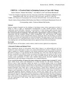
To model dry friction, we propose to use Coulomb’s friction law (see Figure 4) which states that if the tangential response forces f~T are less than the normal force f~n scaled by a friction coefficient µ, objects stick together as tangential displacement δ~T is null. Otherwise, objects slip (δ~T 6= ~0) , and the response forces are scaled back to a dissipative behavior f~T = −µ || f~n || ~T (dynamic friction). As we use an integrated Coulomb model, we are working in displacement, not speed.
Writing constraint laws in this space is often easier than it would be in the motion space, and opens the door to more complex constraints. The constraints space parameters are often not independent, and we need to express the dynamic relationship between them. A mapping function linking the positions in the motion space to the constraints space is often non-linear. In the general case, the problem is reduced to a linear problem using a Jacobian H evaluated at time t around the constraint position. This matrix is used to construct the operator w, that expresses the mechanical coupling in the constraint space: w = HCHT In that expression, matrix C is the compliance matrix, computed as: � C=
Figure 4: Coulomb’s friction law. The reaction force is strictly inside the cone when objects stick together, and on the cone’s border when they slip.
4. Constraints space We have seen that all constraints can be defined by a direction along which a force will be applied in order to respect the constraint. Parameters used on constraint laws: • violation measure (bilateral) • interpenetration measure (unilateral) • tangential displacement, normal force (friction) are defined along the constraint directions. Thus it is much more easier to solve the constraints if we have a direct access to these parameters during the resolution process. Moreover, expressing the behavior of the constrained objects along the constraints directions should enable us to take into account the coupling between the constraints. In [RK00], Ruspini et al. introduce the contact space as the local solution space in which unilateral constraints have to be computed, through the set of parameters that locally describes the relative motion of the bodies during contact and collision. For a pair of bodies interpenetrating, a collision detection algorithm identifies a set of potential contact points, and provides for each of them the contact normal n, perpendicular to the contact geometry. Using the direction n, we can express the relative distance δ f ree between the two contact points. By generalizing this idea to other constraints and their parameters, we introduce the notion of constraint space. In this space, it is possible to express constraints with a finite life span (e.g. collision response constraints, see section 3.2).
M B + +K h2 h
�−1
Its properties are presented in more details in [SDCG08]. M, B and K are respectively the matrices of mass, damping and rigidity. Depending of the nature of the object, this matrix can be obtained easily (rigid objects), with a specific band-matrix solver (wire-like deformable object) or with a precomputation step like in [SDCG08] (3D linear or corotational deformable objects). For real-time simulation of constrained deformable bodies, the number of degrees of freedom is usually much larger than the amount of constraints applied to them. In that context, solving the problem in the constraints space presents the benefit of significantly reducing the size of the system to compute. However, in the case of pure rigid body dynamics, which is out of the scope of this article targeted on constraining both rigid and deformable objects, and if many constraints are applied, a solving strategy in the motion space could be more relevant, as each body typically has no more than 6 DOF. A local strategy consists in first solving the motion of the bodies without applying the constraints (free motion phase), then solving constraints in the constraints space δ = w f + δ f ree , and finally computing a correction motion. Next section describes these issues.
5. Resolution Before coupling, a constraint only needs to compute the correction force depending on the constraint violation (and on the normal force, for friction constraint). This description can be applied for all the constraints, the specifics of this relation describing their behavior. We propose a solution to express the constraint-specific behavior independently from the resolution algorithm. c The Eurographics Association 2008.
Guébert et al. / Unified Processing of Constraints for Interactive Simulation
5.1. System resolution
5.2. Constraint-specific treatment
There must be some preparations before constraints resolution, and the result of the computation needs to be reinjected into the system before integration. We will present here the different steps of our method:
Constraint resolution without coupling consist in computing the response force f in relation to the parameters of the constraint. The violation of the constraints is noted δ f ree before resolution, and δa during the resolution as it can change multiple times if we use iterative methods. Here are examples of this resolution for some of the constraints we want to simulate:
We start by simulating a time-step of the system, in order to see how the bodies would move if there were no constraints at all, hence the name of Free Motion. It is necessary in order to compute the various parameters of the constraints (interpenetration for contact constraints, violation of bilateral constraints, etc.). Figure 5.a shows the initial configuration of two rigid objects linked with a bilateral constraint, before computation of the free motion. Bodies could have been in contact at the previous time-step, or have moved and there can be some potential collision we have to look for. Here, we take for granted that a geometric collision detection process is available. We then create the constraints in response to the collision detection output, and the other constraints defined by the scene, either statically known at the scene design or dynamically created after some predefined events. If needed, additional computation is performed in order to find all the information needed by the constraints for their resolution (in particular, the δ f ree parameter, see Figure 5.b). Once the constraints directions and parameters are expressed, we can define the constraints space, from which the operator w can be deduced. Once all the prerequisites are computed, we then use the constraints solving algorithm, taking into account the mechanical coupling between them. From a time-step to the next one, it is possible to use time coherency to improve computation: by storing constraints results, one can use them as the initial parameters at the next time-step. From the forces computed as the constraints contribution to the system, we define corrective motions for the points where constraints where applied. Finally, system is integrated. We use an implicit Euler solver, as we already computed the rigidity matrices of the bodies for the mechanical coupling of constraints. Figure 5.c shows the result of the constraints resolution for a simple scene.
• Bilateral constraints. Resolving a bilateral constraint consist in adding a force proportional to the violation, and of opposite direction. f = −δa /w • Unilateral constraints. If the violation is negative, the force is proportional to it, else the force is set to zero. if δa < 0 then f = −δa /w else f =0 end • Friction. The constraint is linked to a bilateral or unilateral constraint. When this constraint is solved, the friction constraint get the resulting force, that is considered as the "normal" force. Then, we compute the tangential forces using Coulomb’s friction law as described in 3.3. 5.3. Modified Gauss-Seidel For the complete simulation of a complex system, we need to couple the constraints, as the resolution of one often change the parameters of its neighbors constraints. This will be done by the constraint solving algorithm, using the mechanical coupling expressed in the space we introduced. We use a modified Gauss-Seidel algorithm, but another iterative constraint solver could have been tested (Jacobi, relaxation, etc.), as long as the resolution of a particular constraint can be isolated from the mechanical coupling. Our Gauss-Seidel is very close to the modification done for contacts by Moreau and Jean; we generalize it to all types of constraints. The Gauss-Seidel algorithm has the added benefit of behaving well with redundant constraints like multiple contacts between 2 objects, and converge quite fast. In Figure 6.b we added redundant constraints; the algorithm converge in all cases, the solution and the number of iterations before convergence depend only on the order in which the constraints were defined.
(a) free motion
(b) violation
(c) resolution
Figure 5: Different steps of a bilateral constraint resolution. The dashed outline represent the initial position of the object.
During one iteration, we compute each constraint dimension by blocking all other constraints and summing their contribution relative to the dimension we are considering: (k)
δa i
(k)
ji
(1)
Guébert et al. / Unified Processing of Constraints for Interactive Simulation
Figure 6: Rigid cubes connected together with (a) 2 bilateral constraints represented here as points; (b) 20 overly redundant constraints. The speed of convergence is the same for the two scenes.
(k)
The computation of δa i uses the f j
(k−1)
already been computed, and the f j yet to be updated.
dimensions that have dimensions that have
After the current violation δa i of a particular constraint has been computed, we can call its specific treatment, passing as parameters this violation δa i and the previous force (k−1) fi , which is usually needed for the constraints with friction. The result of a constraint resolution is a new response (k) force fi , replacing immediately the previous one. Note that wi j does not have to be given each time, as it is constant for one system resolution. (k)
(k−1)
We compute the error as err = ∑i wi j ( fi − fi ) and stop iterating the Gauss-Seidel when it goes below a certain tolerance, or a maximum number of iterations has been reached. The modified Gauss-Seidel can be synthesized as: repeat reset error forall constraints dimensions do store previous force for error computation compute δa from Eq. (1) call the constraint-specific treatment save new force compute and add error end until error < tolerance ; This method can handle closed loops as shown in Figure 7, but is restricted to non-conflicting constraints, which should not happen if the they are carefully defined. Note that adapting other iterative algorithms to the proposed method should be straightforward.
Figure 7: A scene where bodies are constrained in a closed loop.
5.4. A note on software architecture On the implementation side, we use the object oriented programming paradigm which enables us to define a general constraint used by the resolution algorithm, and derive from it a family of constraints, each with its own behavior and data. This has shown a few advantages over a global constraints resolution algorithm: Each individual constraint can store data, its own parameters. When it needs to compute the response force created by a constraint, the resolution algorithm only supply δa and f defined at this time of the resolution. The operator w doesn’t change and is known at the start of the constraints resolution. Additional parameters are stored locally by the constraint object for its internal use. For example, contact constraints with friction store their friction coefficient, which can be different for each constraint. It is then possible to simulate contact between objects with various surface friction. Usually, a Gauss-Seidel algorithm computes the resolution one line at a time, each line representing a constraint dimension. It is not a problem for simple contact constraints, or for multiple dimensions bilateral constraints which can be transformed into multiple one-dimensional constraints. However, friction contacts or sliding points with friction need to work with at least 3 dimensions at once, and so the resolution algorithm is usually adapted to this need. We propose that the decision to use one or multiple lines is not for the resolution algorithm to make, but that each constraint will inform the algorithm of its need. This way, simple contact constraints will use one line at a time, whereas c The Eurographics Association 2008.
Guébert et al. / Unified Processing of Constraints for Interactive Simulation
more complex constrains will have access to the additional dimensions they require. One aspect of the previous statement is that we can optimize constraints resolution for faster convergence of the algorithm. What we mean is that for multiple dimensions constraints like 3D fixed point constraint, we will opt for a resolution per 3 by 3 bloc (instead of per line), even if they can be constructed as 3 one-dimension constraints. We compute for all dimensions f = wb −1 δa , with wb the 3 by 3 bloc matrix and wb −1 being precomputed. This approach makes possible the simulation of nonholonomic or nonlinear constraints. We are also not limited to constraints which can be expressed as a simple mathematic relation between responce force and displacement. Contact constraints can be deactivated during resolution if the objects have been separated by other constraints, friction constraints can be sticking or slipping depending of their own parameters. This opens a whole set of possibilities, and we can imagine constraints which completely change their behavior during resolution. The design of the method was thought in order to promote the creation of new types of constraints. Indeed, adding a new constraint is often limited to describing its law of behavior. The constraints resolution algorithm does not need to be changed in any way, as it manipulates only generic constraints. We do not restrain the constraints to abide by strict rules, as they choose their number of dimensions, and the data they need for their resolution. 6. Results We integrated our method into the SOFA framework [SOF], and used the collision detection and integration schemes it proposes. The measures we present for the example scenes were done on a bi-Xeon 2.66Ghz.
Figure 8: Sliding constraints define a direction toward the closest point on the curve.
the boundaries of the current segment, and continue onto the next segment of the curve in this direction. This is done instead of searching only for the closest segment, and allows for complex paths, loops and sharp angles. We detect when the object is at one end of the curve, and depending on the parameters of the scene, either a new unilateral constraint is created preventing the object from falling off the curve, or we disconnect the object from the curve and destroy the sliding constraint of this particular point. A specialization of this sliding constraint has been created, adding friction in the tangential direction, depending on the force pulling the object on the curve. 6.2. Examples The purpose of our method is to be able to represent complex interactions between heterogeneous bodies, for realtime simulations. We first present 2 simple scenes. Figure 9.a shows the use of bilateral constraints, more precisely 3d fixed points, and contact. The top cube is fixed, the others are then attached to each other, all bodies are rigid. Collision detection can create contact constraints, as shown here between the two cubes at the bottom.
6.1. Sliding constraint As a way of testing the framework, we created a new type of constraint: the sliding constraint, whose purpose is to maintain an object on a curve. It is a bilateral constraint, defined between a curve described as a set of connected segments and a set of points which are to be constrained. At each time step, we compute the closest point to the object on the curve, and the tangential direction of the curve at this point. A bilateral constraint is then created along the 2 orthogonal directions (see Figure 8), the violation of the constraint being the distance between the object and the curve. The tangential direction is not constrained, so the object is able to move along the curve during the free motion, and is only projected back to the closest point. During the computation of the projected point, we detect if it would be outside c The Eurographics Association 2008.
Figure 9: (a) Rigid cubes constrained with bilateral constraints. (b) Collision with friction and fixed point constraint.
Figure 9.b illustrate contact constraints with friction. Two rigid cubes are connected with a 3d fixed point constraints, and fall freely on a inclined plane. By varying the friction
Guébert et al. / Unified Processing of Constraints for Interactive Simulation
# of constraints Free motion Collision detection Constraints creation Resolution Movement correction
15 0.6 ms 0.3 ms 0.08 ms 0.02 ms 0.05 ms
Table 1: Measures for the scene of Figure 9.a
coefficient, we can have either slipping or sticking contact. The user can interact with the objects, and stack the cubes as shown here. # of constraints Free motion Collision detection Constraints creation Resolution Movement correction
27 0.2 ms 0.4 ms 0.09 ms 0.9 ms 0.04 ms
Table 2: Measures for the scene of Figure 9.b These 2 scenes are compatible with complete haptic feedback, as the mechanic resolution runs at 1kHz. We finally show a more complex simulation, using all the constraints we introduced, and different types of bodies. Figure 10.b presents the configuration of this scene. We used more detailed, rigid and deformable bodies, sliding on a deformable wire modeled with beams. This cable is fixed at its extremities by bilateral constraints, and collision detection dynamically create contact constraints with friction. This simulation runs at interactive rates, approximately 20 fps. Note that the computations added by our method, namely constraints creation and resolution and movement correction are still relatively fast. The bottleneck in this scene is the collision detection, which is offered by the framework we used. # of constraints Free motion Collision detection Constraints creation Resolution Movement correction
Figure 10: All constraints in a complex scene with deformable and rigid bodies.
60 26 ms 41 ms 3 ms 0.5 ms 2 ms
Table 3: Measures for the scene of Figure 10 Figure 11: The same scene with (a) 2 rigid bodies; (b) 2 deformable models (see dragons’ faces contact). 7. Conclusion We have presented a generalized method for resolving different types of constraints for real-time simulations. We presented how we modified an existing Gauss-Seidel algorithm, with minimal overhead. We have shown that new constraints c The Eurographics Association 2008.
Guébert et al. / Unified Processing of Constraints for Interactive Simulation
of all kinds can easily be added to the framework and that interactive rates are achieved, even for complex interactions. In the future, we would like to continue creating new constraints, for applications in medical simulations, in particular suturing tasks. The high rates at which the mechanic is solved open perspectives in haptic feedback research.
[MJ96] M OREAU J.-J., J EAN M.: Numerical treatment of contact and friction : the contact dynamic method. Engineering Systems Design and Analysis, vol 4 (1996), 201– 208. [Mur97] M URTY K.: Linear complementarity, linear and nonlinear programming. internet edition, 1997.
In the method we presented, the constraints are always destroyed at each time step, and the Gauss-Seidel has no initial guess to start the resolution. We want to investigate the possibility of optimizing the constraints creation and resolution by storing results between time steps.
[RA02] R ENOUF M., A LART P.: Conjugate gradient type algorithms for frictional multi-contact problems: applications to granular materials. Computer Methods in Applied Mechanics and Engineering, 18-20 (2002), 2019– 2041 vol.194.
8. Acknowledgements
[RK00] RUSPINI D., K HATIB O.: A framework for multicontact multi-body dynamic simulation and haptic display. Intelligent Robots and Systems, 2000. (IROS 2000). Proceedings. 2000 IEEE/RSJ International Conference on 2 (2000), 1322–1327 vol.2.
The Authors would like to thank reviewers for useful comments on the submitted work. SOFA development team also provided useful support. This work is partially funded by ANR project VORTISS ANR-2006-MDCA-015 and ANR project Part@ge ANR-06-TLOG-031. References [APS99] A NITESCU M., P OTRA F., S TEWART D.: Timestepping for three-dimentional rigid body dynamics. Computer Methods in Applied Mechanics and Engineering, 177 (1999), 183–197. [Bar89] BARAFF D.: Analytical methods for dynamic simulation of non-penetrating rigid bodies. In SIGGRAPH ’89: Proceedings of the 16th annual conference on Computer graphics and interactive techniques (New York, NY, USA, 1989), ACM, pp. 223–232. [Bar96] BARAFF D.: Linear-time dynamics using lagrange multipliers. In SIGGRAPH ’96: Proceedings of the 23rd annual conference on Computer graphics and interactive techniques (New York, NY, USA, 1996), ACM, pp. 137–146. [DDKA06] D URIEZ C., D UBOIS F., K HEDDAR A., A N DRIOT C.: Realistic haptic rendering of interacting deformable objects in virtual environments. IEEE Transactions on Visualization and Computer Graphics 12, 1 (2006), 36–47. [DLC07] D EQUIDT J., L ENOIR J., C OTIN S.: Interactive contacts resolution using smooth surface representation. In MICCAI (2) (2007), pp. 850–857. [Fea99] F EATHERSTONE R.: A divide-and-conquer articulated-body algorithm for parallel o(log(n)) calculation of rigid-body dynamics. The International Journal of Robotics Research 18, 9 (1999), 876–892. [LF04] L ENOIR J., F ONTENEAU S.: Mixing deformable and rigid-body mechanics simulation. Computer Graphics International, 2004. Proceedings (June 2004), 327– 334. c The Eurographics Association 2008.
[RKC02] R EDON S., K HEDDAR A., C OQUILLART S.: Gauss’ least constraints principle and rigid body simulations. Robotics and Automation, 2002. Proceedings. ICRA ’02. IEEE International Conference on (2002), 517–522 vol.1. [SDCG08] S AUPIN G., D URIEZ C., C OTIN S., G RISONI L.: Efficient contact modeling using compliance warping. In Computer Graphics International Conference (CGI) Istambul, Turkey, (june 2008). [SOF] Simulation open framework architecture. http: //www.sofa-framework.org. [WGW90] W ITKIN A., G LEICHER M., W ELCH W.: Interactive dynamics. SIGGRAPH Comput. Graph. 24, 2 (1990), 11–21.