Given a set of n keys, and an integer i (1 ⤠i ⤠n), the problem of selection is to find ... If a hypercube processor can handle only one edge at any time step, this ...
Unifying Themes for Network Selection1 Sanguthevar Rajasekaran2 Wang Chen Shibu Yooseph Dept. of CIS, Univ. of Pennsylvania Philadelphia, PA 19104 Abstract. In this paper we present efficient deterministic and randomized algorithms for selection on any interconnection network when the number of input keys (n) is ≥ the number of processors (p). Our deterministic algorithm runs on any network in time O( np log log p + Tps log n), where Tps is the time needed for sorting p keys using p processors (assuming that broadcast and prefix computations take time less than or equal to Tps ). As an example, our algorithm √ √ √ runs on a p × p mesh in time O( np log log p + p log n), where n is the input size. This time bound is nearly optimal and significantly better than that of the best existing algorithm when n is large. On the other hand, our randomized algorithm runs in an expected time of O(( np + s s ) log log p) on any network, where Tsparse is the time needed for collecting and Tsparse √ 1−� sorting p sample keys using p processors. (Here � is a constant < 1). On a p × √ √ n p mesh our algorithm runs in an expected O(( p + p) log log p) time, a significant improvement over the deterministic algorithm. We have implemented our randomized algorithm on the Connection Machine CM2. Experimental results obtained are promising. In this paper we also report our implementation details.
1
Introduction
Given a set of n keys, and an integer i (1 ≤ i ≤ n), the problem of selection is to find the ith smallest key in the set. This important comparison problem has an elegant linear time sequential algorithm [1]. Optimal algorithms also exist for certain parallel models like the CRCW PRAM, the comparison tree model, etc. We are interested in solving the selection problem on any interconnection network.
1.1
Models Definition
Though our selection algorithms apply to a general network, we’ll employ the mesh and the hypercube as examples. We assume throughout that n is a polynomial in p. √ √ A mesh connected computer is a p × p square grid where there is a processor at each grid point. Each processor is connected to its four or less neighbors through bidirectional links. It is assumed that in one unit of time a processor can perform a local computation and/or communicate with all its neighbors. A hypercube of dimension � consists of p = 2� nodes (or vertices) and �2�−1 edges. Thus each node in the hypercube can be named with an �-bit binary number. If x is any node in V , then there is a bidirectional link from x to a node y if and only if x and y (considered as binary numbers) differ in exactly one bit position (i.e., the hamming distance between x and y is 1.) Therefore, there are exactly � edges going out of (and coming into) any vertex. If a hypercube processor can handle only one edge at any time step, this version of the hypercube will be called the sequential model. Handling (or processing) an edge here means either sending or receiving a key along that edge. A hypercube model where each processor can process all its incoming and outgoing edges in a unit step is called the parallel model. We assume the sequential model in this paper. 1 This
research was supported in part by an NSF Research Initiation Award CCR-92-09260. current address: Dept. of CIS, Univ. of Florida, Gainesville, FL 32611.
2 Author’s
1.2
Previous Results
Deterministic Selection Krizanc and Narayanan [4] have presented efficient algorithms for se√ n lection on the mesh. Their algorithm runs in time O(min{p log np , max{ p2/3 , p}}). However, they only account for the communication steps in the algorithm. In particular, they discount local computations performed at individual nodes. Plaxton [7] has presented an algorithm for selection out of n elements that runs on a p-node sequential hypercube in time O((n/p) log log p + (Tps + Tpb log p) log(n/p)), where Tps is the time needed for sorting p keys (located one per processor) on a p-processor hypercube, and Tpb is the time needed for broadcasting and summing on a p-node hypercube. He [7] has also proved a lower bound of Ω((n/p) log log p + log p) for selection. For n ≥ p log2 p the lower bound matches the upper bound (to within a multiplicative constant). The only operations allowed on the keys are copying and comparison (for both the upper bound and the lower bound). Randomized Selection Meggido’s [6] algorithm does maximal and median selection in constant time using a linear number of processors on the comparison tree model. Reischuk’s [13] selection algorithm runs in O(1) time using n comparison tree processors. Floyd and Rivest’s [2] sequential algorithm takes n+min(i, n−i)+o(n) time. In [8], Rajasekaran has presented randomized algorithms for selection on the hypercube (on both the sequential and parallel versions). In [9], Rajasekaran also presents optimal or very nearly optimal randomized algorithms for selection on the mesh with fixed as well as reconfigurable buses. Randomized selection algorithms for the star graph have been given by Rajasekaran and Wei [12]. Rajasekaran and Sen [11] give an O(1) time n processor maximal selection algorithm for the CRCW PRAM model. Krizanc and Narayanan [3] have presented optimal algorithms for selection on the mesh connected computers. All these results hold for the worst case input with high probability. For an extensive survey of randomized selection algorithms, see [10].
1.3
New Results
Deterministic Selection On any p-node network, our deterministic selection algorithm runs in time O( np log log p + Tps log n), where Tps is the time needed for sorting p numbers using p processors. √ On the mesh this algorithm runs in time O( np log log p + p log n), taking into account all √ n local computations performed. Since Ω( p + p) is a trivial lower bound, our algorithm is very nearly optimal. If we neglect the time spent on local computations, the run time of our algorithm √ √ will be O( p log n). Clearly, this time bound is close to the trivial lower bound of Ω( p). For all n > p7/6 log p, our algorithm will have a much better run time than that of [4]. The same algorithm runs in time O( np log log p + log2 p log log p) on the hypercube. The run time of our algorithm very nearly matches that of Plaxton [7]. But if a better sorting algorithm is discovered, the run time of our algorithm will improve somewhat, whereas [7]’s algorithm does not seem to improve. Randomized Selection Our randomized algorithm runs in an expected time of s s O(( np + Tsparse ) log log p) on any network with p nodes, where Tsparse is the time needed for col1−� lecting and sorting p sample keys using p processors. (Here � is a constant < 1). On the mesh √ this algorithm runs in an expected O(( np + p) log log p) time, a significant improvement over the deterministic algorithm. On the hypercube also, our algorithm has a better run time than that of [7], as has already been shown in [8]. We have implemented our randomized algorithm on the Connection Machine CM2. We report our experimental results in this paper.
2
Preliminary Facts
2.1
Sorting
We make use of existing sorting algorithms. The following theorem is due to Schnorr and Shamir [14]: √ Lemma 2.1 Sorting on a p-node mesh can be completed in time O( p), the queue size being O(1) if there is a single key input at each node. Proof of the following Lemma due to Cypher and Plaxton can be found in [5]. Lemma 2.2 Sorting on a p-node hypercube can be completed in time O(log p log log p).
2.2
Broadcasting and Summing
Broadcasting is the operation of a single processor sending some information to all the other processors. The prefix sums problem is this: Processor v in a p-node hypercube has an integer kv , for �v 1 ≤ v ≤ p. Processor v has to compute j=1 kj . √ Lemma 2.3 Both broadcasting and prefix sums problem can be completed in O( p) steps on a p-node mesh. Lemma 2.4 Both broadcasting and prefix sums problem can be completed in O(log p) steps on a p-node sequential hypercube.
3 3.1
Deterministic Selection Summary of our Technique
The basic idea behind our algorithm is the same as the one employed in [1]. The sequential algorithm of [1] partitions the input into groups (of say 5), finds the median of each group, and computes recursively the median (call it M ) of these group medians. Then the rank rM of M in the input is computed and as a result, all the elements from the input which are either ≤ M or > M are dropped, depending on whether i > M or i ≤ M , respectively. Finally, an appropriate selection is performed from out of the remaining keys recursively. An easy analysis will reveal that the run time of this algorithm is O(n). The same algorithm can be used in parallel, for instance on a PRAM, to obtain an optimal algorithm. If one has to employ this algorithm on a network, it seems like one has to perform periodic load balancing (i.e., distribute remaining keys uniformly among the processors). In [7], an algorithm is given which identifies an M for splitting the input upon, which automatically ensures (approximate) load balancing. That is, at least one half of the keys from any node will be eliminated every time the remaining keys are split. In this paper we introduce a different approach. We employ the same algorithm as that of [1], with a twist. To begin with each node has exactly np keys. As the algorithm proceeds, keys get dropped from future consideration. We never perform any load balancing. The remaining keys from each node will form the groups. We identify the median of each group. Instead of picking the median of these medians as the splitter key M , we choose a weighted median of these medians. Each group median is weighted with the number of remaining keys in that node. This simple algorithm (with some minor modifications) yields the stated results.
3.2
Selection on the Mesh
√ √ √ In this section we show that selection can be done in time O( np log log p + p log n) on a p × p mesh, the input size being n. To begin with, there are exactly np keys at each node. We need to find the ith smallest key.
Algorithm I N := n Step 0. if log(n/p) is ≤ log log p then sort the elements at each node else partition the keys at each node into log p equal parts such that keys in one part will be ≤ keys in the parts to the right. repeat Step 1. In parallel find the median of keys at each node. Let Mq be the median and Nq be the number of remaining keys at node q, 1 ≤ q ≤ p. Step 2. Find the weighted median of M1 , M2 , . . . , Mp where key Mq has a weight of Nq , 1 ≤ q ≤ p. Let M be the weighted median. Step 3. Count the rank rM of M from out of all the remaining keys. Step 4. if i ≤ rM then eliminate all remaining keys that are > M else eliminate all keys that are ≤ M . Step 5. Compute E, the number of keys eliminated. if i > rM then i := i − E; N := N − E. until N ≤ c, c being a constant. Output the ith smallest key from out of remaining keys. Analysis. Step 0 takes time np min{log(n/p) , log log p}. At the end of Step 0, the keys in any node have been partitioned into nearly log p nearly equal parts. Call each such part as a block. n In Step 1, we could find the median at any node in O(log p + p log p ) time. In Step 2, we could � sort the medians and thereby compute the weighted median. If M1 , M2� , . . . , Mp� is the sorted order � � N � of the medians, then, we need to identify j such that jk=1 Nk� ≥ N2 and j−1 k=1 Nk < 2 . Such a j can be computed with an additional prefix computation. Thus M , the weighted median, can be √ √ n identified in time O( p) (c.f. Lemmas 2.1 and 2.3). Step 3 takes O( p log p) time. Step 4 also p + √ √ n + p) time. Step 5 takes O( p) time, since it involves just a prefix operation. takes O( p log p √ n Thus each run of the repeat loop takes O( p log + p) time. p How many keys will get eliminated in each run of the repeat loop? Assume that i ≥ rM in a given� run. � (The other case can be argued similarly). The number of keys eliminated is at least �j Nk� which is ≥ N4 . Therefore, it follows that the repeat loop will be executed O(log n) times. k=1 2 Thus we get (assuming that log n is asymptotically the same as log p): Theorem 3.1 Selection on a p-node square mesh can be performed in time O( np log log p +
√
p log n).
Often times, the time needed for communication far outweighs the time needed for local computations in a network based computer. Thus it may be reasonable to neglect local computations. In [3], Krizanc and Narayanan make this assumption to derive the run time of their algorithm. It is easy to compute the run time of our algorithm under this assumption and obtain the following: √ Theorem 3.2 If local computations are neglected, the run time of our algorithm is O( p log n).
3.3
Selection on the Hypercube
Our selection algorithm when applied on the hypercube yields a run time of O( np log log p + Tps log n), where Tps is the time needed to sort p keys on a p-node hypercube. With the currently best known value for Tps , the run time of our algorithm very nearly matches that of [7]. However, if a better sorting algorithm is discovered, the run time of our algorithm will improve. Our algorithm is also somewhat simpler than that of [7]’s. Here also, there are np keys to begin with at each node and we have to identify the ith smallest key.
Algorithm II N := n Step 0. if log(n/p) is ≤ log log p then sort the elements at each node else partition the keys at each node into log p equal parts such that keys in one part will be ≤ keys in parts to the right. repeat Step 1. In parallel find the median of keys at each node. Let Mq be the median and Nq be the number of remaining keys at node q, 1 ≤ q ≤ p. Step 2. Find the weighted median of M1 , M2 , . . . , Mp where key Mq has a weight of Nq , 1 ≤ q ≤ p. Let M be the weighted median. Step 3. Count the rank rM of M from out of all the remaining keys. Step 4. if i ≤ rM then eliminate all remaining keys that are > M else eliminate all keys that are ≤ M . Step 5. Compute E, the number of keys eliminated. if i > rM then i := i − E; N := N − E. until N ≤ c, c being a constant. Output the ith smallest key from out of remaining keys. Analysis. Step 0 takes time np min{log(n/p) , log log p}. At the end of Step 0, the keys in any node have been partitioned into nearly log p nearly equal parts. Call each such part as a block. n Step 1 takes time O(log p + p log p ) just as in the mesh algorithm. In Step 2, we could employ a sorting followed by a prefix computation in order to identify the weighted median. Thus Step 2 will n take time O(Tps + log p) (c.f. Lemmas 2.2 and 2.4). Step 3 takes O( p log p + log p) time. Step 4 also n takes O( p log p + log p) time. Step 5 can be completed in O(log p) time, using a prefix operation. n s Therefore, each run of the repeat loop takes O( p log p + Tp + log p) time. At least a constant fraction of the keys get eliminated during each run of the repeat loop (for the same reason as in the mesh algorithm). Therefore, assuming that log n is asymptotically the same as log p, the run time of the algorithm is O( np log log p + Tps log n). As a result, we get: Theorem 3.3 Selection on a p-node hypercube can be performed in time O( np log log p + Tps log n), where Tps is the time needed for sorting and n is the input size. The following theorem is also clear: Theorem 3.4 Selection on a p-node hypercube can be performed in time O( np log log p + Tpw log n), where Tpw is the time needed for computing the weighted median of p numbers on a p-node hypercube. Our selection algorithm can be implemented on any network to obtain a very nearly optimal run time. The following theorem assumes that broadcast and prefix computations take time less than or equal to the time needed for sorting: Theorem 3.5 Selection can be performed in time O( np log log p + Tps log n) on any network with p processors, where Tps is the time needed for sorting p numbers using p processors.
4 4.1
A Randomized Selection Algorithm Summary
The algorithm we present can be thought of as an extension of the algorithms given in [2, 8]. Given is a set X of n keys and an integer i, 1 ≤ i ≤ n. Assume the keys are distinct (without loss of
generality). We need to identify the ith smallest key. We sample a set S of o(n) keys at random. Sort the set S. Let l be the key in S with rank m = �i(|S|/n) . We will expect the rank of l in X to be roughly i. We identify two keys l1 and l2 in S whose ranks in S are m − δ and m + δ respectively, δ being a ‘small’ integer, such that the rank of l1 in X is < i, and the rank of l2 in X is > i, with high probability. Next we eliminate all the keys in X which are either < l1 or > l2 . We repeat this phase of sampling and elimination until the number of keys remaining is ‘small’. Finally, we concentrate and sort the remaining keys. An appropriate selection is performed on the surviving keys. The following sampling lemma from [10] will be used in our analyses. Let S = {k1 , k2 , . . . , ks } be a random sample from a set Y of cardinality N . Let ‘select(Y, i)’ stand for the ith smallest element of Y for any integer i. Also let k1� , k2� , . . . , ks� be the sorted order of the sample S. If ri is the rank of ki� in Y and if |S| = s, the following lemma [10] provides a high probability confidence interval for ri . � � √ N√ log N < N −α . Lemma 4.1 For every α, Prob. |ri − i Ns | > 3α √ s
4.2
The Algorithm
s Now we present details of our algorithm. The algorithm runs in an expected O(( np +Tsparse ) log log p) s time on any p-node interconnection network. Here Tsparse is the time needed for concentrating and sorting p1−� sample keys using p processors, � being a constant (dependent on the network) less than 1. This expectation is over the space of outcomes for the coin flips and not over the space of possible inputs. To begin with, each key is alive.
Algorithm R-Select N := n; (* N at any time is the number of alive keys *) repeat forever Step 0 If N is < C then quit and go to Step 7 (C being a constant). Step 1 Each processor flips an N � -sided coin for each one of its alive keys. An alive key gets included in the random sample, S, with probability N −� . This step takes np time and with high probability O(N 1−� ) keys (from among all the processors) will be in the random sample. Step 2 p processors perform a prefix sums operation to compute the number of keys in the sample. Let q be this number. If q is not in the range [0.5N 1−� , 1.5N 1−� ] go to Step 1. Step 3 Concentrate the sample keys. Step� 4 �Sort the sample keys. Pick keys l1 and l2 from S with √ ranks √ iq and N + d q log N , respectively, d being a constant > 3α.
� iq � N
√ − d q log N
Step 5 Broadcast l1 and l2 to all the processors in the network. The key to be selected will have a value in the range [l1 , l2 ] w.h.p. Step 6 Count the number, r, of alive keys with a value in the range [l1 , l2 ]. Also count the number of alive keys with a value < l1 . Let this count √ be t. If i is not in the interval (t, t + r] or if r is �= O(N (1+�)/2 log N ) go to Step 1 else kill (i.e., delete) all the alive keys with a value < l1 or > l2 . Set i := i − t. Set N := r.
end repeat; Step 7 Concentrate the alive keys and output the key of rank i. Analysis. We perform the analysis for the mesh. A choice of � = 9/10 is appropriate for a mesh. Similar analysis can be employed for any network. We first obtain an upper bound for the run time of each phase of the repeat loop followed by an estimate on the number of times the repeat loop will be executed. √ In any phase, Steps 0 and 5 take O( p) time each. Step 1 takes np time. Prefix in Steps 2 and √ 6 can be performed in O( np + p) time. The number of sample keys is B(N, N1� ). This means, using Chernoff bounds, that the number of sample keys will be in the range [0.5N 1−� , 1.5N 1−�] with probability ≥ 1 − 12 N −α for any fixed α ≥ 1. Let A be the event: ‘q lies in the interval [0.5N 1−� , 1.5N 1−� ]’. Let B be the event: ‘the key to be selected lies in the interval [l1 , l2 ] and √ this interval is of size O(N (1+�)/2 log N )’. We can make Prob.[B/A] ≥ 1 − 12 N −α , by choosing an appropriate constant d. Therefore, Prob.[A B] is ≥ 1 − N −α . √ Thus, any phase of the repeat loop (excepting Steps 3 and 4) runs in a total of O( np + p) time with probability ≥ (1 − N −α ), N being the number of alive keys at the beginning of this phase. √ Therefore, the expected run time of any phase (with the exception of Steps 3 and 4) is O( np + p). Next we show that the expected number of times that the repeat loop is executed is O(log log p) = O(log log n). If there are N alive elements at the beginning of any iteration of the repeat loop, then √ � √N � �� ) (for any fixed the number of elements at the end of this iteration is O( log N ) = O(N N 1−� �� > (1 + �)/2; c.f. Lemma 4.1; here the high probability is with respect to N ). This implies that the expected number of times the repeat loop is executed is O(log log n) = O(log log p). √ We show that Steps 3 and 4 take a total expected time of O(( np + p) log log p) over all the phases. Thus we obtain: √ Theorem 4.1 Selection out of n elements can be performed in an expected O( np log log p+ p log log p) time on a p-node mesh. Along the same lines we could get: s Theorem 4.2 Selection out of n elements can be performed in an expected O(( np +Tsparse ) log log p) time on any p-node interconnection network.
[8].
5
On the sequential hypercube, this time bound is O(( np + log p) log log p), as has been shown in
Implementation Results
A slight variant of algorithm R-Select has been implemented on the Connection Machine CM2. CM2 located in the CIS department of UPenn has 4096 processing elements and is a SIMD machine. Each processing element is limited in capacity and can compute any function that maps three bits into two bits.The underlying communication network is a hypercube. Nearest neighbor as well as global communications (i.e., partial permutations) are supported. Special purpose hardware computes functions such as scan, broadcast, etc. CM2 supports virtual processors as well. There is also a built-in function called rank for ranking elements in a given sequence. In fact, in this draft we are comparing the performance of our program with that of rank. Though this may not be an acceptable comparison, there is no other appropriate built-in function. However, we are currently implementing our deterministic algorithm also. Next we give some details of our implementation. We have defined a parallel variable with n elements to store the input of n numbers. This amounts to using a (virtual) machine with n processing elements. To begin with each input number is alive. In any phase of the program (i.e., in any run of the repeat loop), we choose nearly 64 sample keys randomly, concentrate, and sort them. We pick two elements from the sample whose ranks are ( Ni − t)64 and ( Ni + t)64. Here N is the
Seconds
2.0 x
rank
+
R-Select
1.5
1.0
x
0.5
x +
x x x + +
+
1 2
4
+
Input size 8
16
32
X 2
13
Figure 1: Execution Times of R-Select on CM2 number of alive keys and t is a fraction that has been experimentally adjusted for best performance. 1 For the input sizes tried, a value between 12 and 18 seems appropriate for t. In our first implementation we used rank to sort the sample keys. Even though the sample size was very small, rank took a considerable amount of time to sort them. So, we used the following simple algorithm: Compare all pairs of numbers and thereby compute the rank of each number. This sort is very fast since it involves only a few scan operations. After having chosen the two keys �1 and �2 , we broadcast them and delete appropriate keys to complete a phase of the program. After each phase of our program, the number of surviving keys will dramatically decrease. But with the chosen shape for the parallel variables, the run time of any phase was nearly the same as that of the previous phase. In order to overcome this problem, we chose to perform a load balancing operation in every phase. This was done by dynamic allocation and deallocation of parallel variables and a scan operation to concentrate surviving keys into a smaller parallel variable. Our experimental results are summarized in Figure 1. We ran the program on various input sizes ranging from 8192 to 262,144. Inputs were generated randomly. The run time shown is averaged over 20 independent runs. As is clear from the Figure 1, R-Select outperforms rank especially when the input size is large. Our code has not been optimized; performance should improve with any such optimization. Currently we are implementing our deterministic algorithm also on CM2. It would be interesting to compare these two programs.
6
Conclusions
In this paper we have presented deterministic and randomized algorithms for selection on any network. On the mesh and the hypercube, for example, our algorithms have better time bounds than previously best known algorithms. Our randomized algorithm has been implemented on CM2; the results are promising.
Acknowledgements The first author would like to thank Danny Krizanc for many stimulating interchange of ideas.
References [1] M. Blum, R. Floyd, V.R. Pratt, R. Rivest, and R. Tarjan, Time Bounds for Selection, Journal of Computer and System Science, 7(4), 1972, pp. 448-461. [2] R.W. Floyd, and R.L. Rivest, Expected Time Bounds for Selection, Communications of the ACM, Vol. 18, No.3, 1975, pp. 165-172. [3] D. Krizanc, and L. Narayanan, Optimal Algorithms for Selection on a Mesh-Connected Processor Array, Proc. Symposium on Parallel and Distributed Processing, 1992. [4] D. Krizanc and L. Narayanan, Multi-packet Selection on a Mesh-Connected Processor Array, in Proc. International Parallel Processing Symposium, 1992. [5] T. Leighton, Introduction to Parallel Algorithms and Architectures: Arrays–Trees–Hypercube, Morgan-Kaufmann Publishers, 1992. [6] N. Meggido, Parallel Algorithms for Finding the Maximum and the Median Almost Surely in Constant Time, Preliminary Report, CS Department, Carnegie-Mellon University, Pittsburg, PA, Oct. 1982. [7] C.G. Plaxton, Efficient Computation on Sparse Interconnection Networks, Ph. D. Thesis, Department of Computer Science, Stanford University, 1989. [8] S. Rajasekaran, Randomized Parallel Selection, Proc. Symposium on Foundations of Software Technology and Theoretical Computer Science, 1990, pp. 215-224. [9] S. Rajasekaran, Mesh Connected Computers with Fixed and Reconfigurable Buses: Packet Routing, Sorting, and Selection, in Proc. First Annual European Symposium on Algorithms, 1993. [10] S. Rajasekaran and J.H. Reif, Derivation of Randomized Sorting and Selection Algorithms, Parallel Algorithm Derivation and Program Transformation, Edited by R. Paige, J.H. Reif, and R. Wachter, Kluwer Academic Publishers, 1993, pp. 187-205. [11] S. Rajasekaran, and S. Sen, Random Sampling Techniques and Parallel Algorithms Design, in Synthesis of Parallel Algorithms, Editor: J.H. Reif, Morgan-Kaufman Publishers, 1993, pp. 411-451. [12] S. Rajasekaran and D.S.L. Wei, Selection, Routing, and Sorting on the Star Graph, in Proc. International Parallel Processing Symposium, pp. 661-665, April 1993. [13] R. Reischuk, Probabilistic Parallel Algorithms for Sorting and Selection, SIAM Journal of Computing, Vol. 14, No. 2, 1985, pp. 396-409. [14] C. Schnorr and A. Shamir, An Optimal Sorting Algorithm for Mesh-Connected Computers, in Proc. ACM Symposium on Theory of Computing, 1986, pp. 255-263.
APPENDIX A: Chernoff Bounds Lemma A.1 If X is binomial with parameters (n, p), and m > np is an integer, then � np �m em−np . P robability(X ≥ m) ≤ m Also, and for all 0 < � < 1.
(1)
P robability(X ≤ �(1 − �)pn�) ≤ exp(−�2 np/2)
(2)
P robability(X ≥ �(1 + �)np ) ≤ exp(−�2 np/3)
(3)