testing for the presence of a unit root in a time series using the Covariate Augmented ... still probably the Augmented Dickey-Fuller (ADF) test (Dickey and Fuller ...
Unit Root CADF Testing with R Claudio Lupi University of Molise
Abstract This introduction to the CADFtest package is a (slightly) modified version of Lupi (2009), published in the Journal of Statistical Software. CADFtest is an R package for testing for the presence of a unit root in a time series using the Covariate Augmented Dickey-Fuller (CADF) test proposed in Hansen (1995b). The procedures presented here are user friendly, allow fully automatic model specification, and allow computation of the asymptotic p values of the test.
Keywords: unit root, stationary covariates, asymptotic p values, R.
1. Introduction and statistical background Testing for a unit root is a frequent problem in macroeconomic modeling and forecasting. Although many tests have been developed so far, the practitioner’s workhorse in this field is still probably the Augmented Dickey-Fuller (ADF) test (Dickey and Fuller 1979, 1981; Said and Dickey 1984), which is known to have good size but low power under many conditions.1 However, the literature on unit root testing has largely proceeded in a univariate framework, with notable exceptions being represented by the panel unit root tests (see Choi 2006b, for a recent survey). In fact, reality is hardly univariate at all and, although univariate representations of multivariate time series exist (see e.g., Zellner and Palm 1974), nevertheless reckoning explicitly the multivariate nature of most economic time series can in principle lead to better testing procedures. In a seminal paper Hansen (1995b) suggests that, when testing for a unit root, a viable way to exploit the information embodied in related series and increase power is to consider stationary covariates in an otherwise conventional ADF framework. Unless the variable of interest is independent of the stationary covariates considered in the analysis, by the Neyman-Pearson lemma the most powerful test makes use of the information embodied in the stationary covariates themselves (Hansen 1995b, p. 1152). As a consequence, not considering the multivariate dimension of the problem leads to a loss in the power of the test. Using covariates also allows to some extent to couple unit root testing and economic theory, because economic theory can be used as a guideline to chose the appropriate covariates to be included in the analysis (see e.g., Amara and Papell 2006; Elliott and Pesavento 2006), although other approaches can be used as well (Lee and Tsong 2009). Formally, Hansen (1995b) considers a univariate time series yt composed of a deterministic 1
However, large negative MA components are well known to have adverse effects on the size of the ADF test (see e.g., Schwert 1989). An interesting summary of many Monte Carlo results on different unit root tests can be found in Stock (1994). Haldrup and Jansson (2006) is a recent survey of the methods proposed to improve the size and the power of unit roots tests.
2
Unit Root CADF Testing with R
and a stochastic component such that yt = dt + st a(L)∆st = δst−1 + vt 0
vt = b(L) (∆xt − µ∆x ) + et
(1) (2) (3)
where dt is the deterministic term (usually a constant or a constant and a linear trend), a(L) := (1 − a1 L − a2 L2 − . . . − ap Lp ) is a polynomial in the lag operator L, ∆xt is a vector of stationary covariates, µ∆x := E(∆x), b(L) := (bq2 L−q2 + . . . + bq1 Lq1 ) is a polynomial where both leads and lags are� allowed � for. Furthermore, the long-run (zero-frequency) covariance P∞ 0 matrix Ω := k=−∞ E �t �t−k , with �t := (vt , et )0 can be defined, from which the long-run squared correlation between vt and et , ρ2 , can be derived. When ∆xt has no explicative power on the long-run movement of vt , then ρ2 ≈ 1. On the contrary, when ∆xt explains nearly all the zero-frequency variability of vt , then ρ2 ≈ 0. The case ρ2 = 0 is ruled out for technical reasons (see Hansen 1995b, p. 1151). It should be noted that this restriction excludes the possibility that the variable yt be cointegrated with the cumulated stationary covariate(s). As with the ADF test, Hansen’s CADF test is based on different models, according to the different deterministic kernels that the investigator may wish to consider. For example, the model with constant and linear trend is a(L)∆yt = µ + θ t + δyt−1 + b(L)0 ∆xt + et .
(4)
d Similarly to the conventional ADF test, the CADF test is based on the t-statistic for δ, t(δ), with the null hypothesis being that a unit root is present, i.e. H0 : δ = 0, against the one-sided alternative H1 : δ < 0. Hansen (1995b) refers to the test statistic as the CADF(p, q1 , q2 ) statistic.
Hansen (1995b, p. 1154) proves that under the unit-root null, if conventional weak dependence d in the model without deterministic terms is such that and moment restrictions hold, t(δ) R1 � �1/2 W dW 2 d t(δ) ⇒ ρ �R0 N (0, 1) �1/2 + 1 − ρ 1 2 0
(5)
W
where ⇒ denotes weak convergence, W is a standard Wiener process, and N (0, 1) is a standard normal independent of W . It is interesting to note that (5) is the distribution of a weighted sum of a Dickey-Fuller and a standard normal random variable. If a model with constant or a model with constant and trend are considered, the standard Wiener process W in (5) has to be replaced by a demeaned or a detrended Wiener process, respectively. Note that the asymptotic distribution of the test statistic depends on the nuisance parameter ρ2 but, provided ρ2 is given, it can be simulated using standard techniques (see e.g., Hatanaka 1996). Hansen (1995b, p. 1155) provides the asymptotic critical values of the test, while here we offer a practical way to compute its p values. Hansen’s CADF test is firmly rooted in the ADF tradition and for this reason it can be more familiar and attractive to practitioners than other tests, although Elliott and Jansson (2003) show that Hansen’s CADF test is not the point optimal test in general. Feasible point optimal tests in the presence of deterministic components are developed in Elliott and Jansson (2003). A quite different approach is used in this case, the feasible tests being based on VAR models.
Claudio Lupi
3
However, Monte Carlo simulations reported in Elliott and Jansson (2003) suggest that power gains with respect to Hansen’s CADF test can be obtained at the cost of slightly worse size performances. In this paper we present the R (R Development Core Team 2009) package CADFtest that allows users to perform Hansen’s CADF unit root test easily. The main function CADFtest() returns a CADFtest class object that not only contains the test statistic, but also its asymptotic p value and many other useful details. In fact, the class CADFtest inherits from the class htest,2 so that no special print() method is needed. However, dedicated summary() and plot() methods have been developed in order to allow the user to analyze the test results more in detail. A specialized update() method is also available that ease testing using different options. The remainder of the paper is structured as follows: Section 2 discusses the way Hansen’s CADF test has been implemented in the function CADFtest(), and some applications are illustrated in Section 3. In Section 4, the method to compute the asymptotic p values is illustrated in detail along with the use of the function CADFpvalues(). Section 5 offers some comparisons with other existing R packages performing the ADF test. A summary is offered in Section 6.
2. Implementation and use of the function CADFtest() In principle, carrying out Hansen’s CADF test is no more complicated than carrying out an ordinary ADF test. What makes things more complicated is the presence of the nuisance parameter ρ2 in the asymptotic distribution (5). In fact, a consistent estimate of ρ2 has to be derived in order to choose the correct asymptotic critical value and/or to compute the correct asymptotic p value of the test. The problem is solved into two steps. First, eˆt and vˆt are derived; then, their long-run covariance matrix Ω is estimated using a HAC covariance estimator (see e.g., Andrews 1991; Zeileis 2004, 2006; Kleiber and Zeileis 2008). Once the kind of model (no constant, with constant, with constant and trend) has been chosen, using CADFtest() the investigator can either set the polynomial orders p, q2 and q1 to fixed values, or can decide the maximum value for each and let the procedure to select and estimate the model according to different information criteria. In order to estimate ρ2 it is necessary to estimate et and vt first. For example, if the model with constant and trend (4) is used, then et and vt are estimated as d d 0 ∆x eˆt = a(L)∆y ˆ∗ − θˆ t − δˆτ yt−1 − b(L) t−µ t 0�
�
d ∆x − ∆x + eˆ vˆt = b(L) t t
(6) (7)
where “b” denote parameters estimated by ordinary least squares and ∆x is the sample average of ∆xt . Once eˆt and vˆt have been computed, a kernel-based HAC covariance estimator (Andrews 1991) is used to estimate Ω and hence ρ2 . In order to estimate ρ2 in a rather flexible way, in CADFtest() the kernHAC() function included in the sandwich package (Zeileis 2004, 2006) is used. This allows the investigator to chose the kernel to be applied, the bandwidth, and if and how prewhitening should be performed. Differently from Hansen (1995b) where a Parzen kernel without prewhitening is used, the default choice in CADFtest() is a quadratic 2
A fairly detailed description of the htest class can be gathered from within R by typing ?t.test.
4
Unit Root CADF Testing with R
spectral kernel with VAR(1) prewhitening. The bandwidth is adaptively chosen using the method proposed in Andrews (1991), but the user is free to change any of these default choices. The usage of the function is extremely simple: CADFtest(model, X = NULL, type = c("trend", "drift", "none"), data = list(), max.lag.y = 1, min.lag.X = 0, max.lag.X = 0, dname = NULL, criterion = c("none", "BIC", "AIC", "HQC", "MAIC"), ...) The minimal required input is CADFtest(y), where y can be either a vector or a time series. However, if no stationary covariate is specified, an ordinary ADF test is performed. In fact, the ordinary ADF test can be carried out with R using other existing packages such as fUnitRoots (Wuertz 2009), tseries (Trapletti 2009) and urca (Pfaff 2008). In this respect there would be no need to add one further package. However, given that the ADF test can be seen as a particular case of the more general CADF test, it seems logical to leave the user the opportunity to carry out both tests in the same framework, using the same conventions and allowing for the computation of the test p values. Furthermore, as will be shown in section 3, the interface to CADFtest() is very flexible and intuitive, and the results are easy to read: this can make carrying out conventional ADF tests using CADFtest() very appealing. As far as the computation of the p values of the ADF test is concerned, CADFtest() exploits the facilities offered by punitroots() implemented in the package urca (Pfaff 2008) that uses the method proposed in MacKinnon (1994, 1996). In principle, it would have been possible (and easy) to use the function CADFpvalues() described in detail in section 4, but given that MacKinnon (1996) describes a method to compute approximate finite sample, rather than asymptotic, p values, it seems fair to refer directly to a function that implements this procedure. However, note that MacKinnon (1996) derives the finite sample p values for Gaussian data: in non-Gaussian settings the finite sample p values are not necessarily more accurate than the asymptotic ones. All the arguments, with the exception of min.lag.X and max.lag.X that are relevant only when a CADF test is carried out, work irrespective of the test being ADF or CADF. However, if a proper CADF test has to be performed, at least a stationary covariate must be passed to the procedure. The covariates are passed in a very simple way, using a formula (model) statement. For example, suppose we want to test the variable y using x1 and x2 as stationary covariates: if the other default options are accepted, then it is sufficient to specify CADFtest(y ~ x1 + x2). Note that the formula that is passed as argument to the CADFtest() function is not the complete model to be used, but it just indicates which variable has to be tested for a unit root (y) and which are to be used as stationary covariates in the test (x1 and x2). A formula statement can be used also to specify an ordinary ADF test by typing CADFtest(y ~ 1), where the term “1” does not imply that a model with constant will be used, but it simply means that no stationary covariate is passed to the procedure (the deterministic kernel is always defined by the argument type described below). Other arguments are used to specify the deterministic kernel to be used in the model (type), the lead and lag orders (max.lag.y, min.lag.X, max.lag.X), and if the model has to be fixed or selected using a criterion such as "AIC" (Akaike 1973), "BIC" (Schwarz 1978), "HQC" (Hannan and Quinn 1979) or "MAIC" (Ng and Perron 2001). Indeed, given that a number of competing models with potentially many regressors have to be compared, information criteria offer a handy solution. Furthermore, Hall (1994) shows that when the data are generated by
Claudio Lupi
5
an ARIMA(p0 , 1, 0) process, then the distribution of the ADF test statistic under the null converges asymptotically to the correct distribution when the number of lags in the empirical model is determined by using either the AIC, the BIC, or the HQC. On the other hand, Ng and Perron (2001) argue that standard information criteria should be modified to take into account the fact that the series are I(1) under the null and propose their modified AIC (MAIC) that should be more robust in the presence of negative moving-average errors. Ng and Perron’s MAIC is computed by CADFtest() in the OLS-detrended version suggested by Perron and Qu (2007). However, notice that although the MAIC should in principle work well also in the CADF framework, its usefulness has been proved only in the simpler ADF context. When no stationary covariate is passed to the procedure, then lag selection is obviously limited to the lags of ∆yt , but when a proper CADF test is performed, then model selection implies the joint determination of the lags of the differenced dependent variable and the leads and lags of the stationary covariates as well. If criterion = "none" (the default choice) is specified, no automatic model selection is performed and the lag orders are fixed to the values passed to the procedure. In particular, max.lag.y corresponds to p, the lag order of a(L) in (4), and it is set to 1 by default: it can be set equal to 0 or to a positive integer. min.lag.X corresponds to q2 , the maximum lead in b(L) in (4), and it is equal to 0 by default: if modified, it must be set equal to a negative integer (a negative lag is a lead). max.lag.X correspond to q1 , the maximum lag in b(L) in (4), and the default choice is 0: if modified, it must be set equal to a positive integer. If criterion is different from "none", then all the models with lags polynomials up to the specified orders (of both the y and the covariates) are estimated and the final model to be used is selected on the basis of the chosen criterion. The deterministic components to be used in the model are specified using the conventions utilized in the R package urca (Pfaff 2008). The default value (type = "trend") implies that the model with constant and trend (4) is used. If type = "drift" or type = "none" is specified, then the model with constant or the model without deterministic components are utilized. data is the data set to be used and dname is the name of data: in general there is no need to change dname, given that it is automatically computed by the function itself, unless one wants to indicate for example that a specific data set has been used. Further arguments can be passed to the procedure to control the parameters to be used in the HAC covariance estimation. These further arguments can be passed using the conventions valid for the command kernHAC() (see the package sandwich: Zeileis 2004, 2006). If Hansen’s results have to be replicated, then kernel = "Parzen" and prewhite = FALSE have to be specified, otherwise a quadratic spectral kernel with VAR(1) prewhitening is used by default. The function CADFtest() returns an object of class CADFtest containing the test statistic (statistic), the p value of the test (p.value), the lag structure of the selected model (max.lag.y, min.lag.X, max.lag.X), the value of the information criteria (AIC, BIC, HQC, MAIC), the estimated value of ρ2 (parameter), and the full estimated model (est.model). Other returned information concern the nature of the test (either CADF or ADF) stored in method, the name of data used (data.name), the value of δ under the null (null.value), the description of the alternative (alternative) and the estimated value of δ (estimate). A summary of the test can be obtained just by using a print() command. Given that the class CADFtest inherits from the class htest, the print() command produces the standard R output of the htest class. However, the summary() command is also allowed that returns a more detailed account of the test results. For greater flexibility, print() can be applied
6
Unit Root CADF Testing with R
to a CADFtestsummary object (produced by summary()) to control further printing options. For example, the number of significant digits can be controlled by digits, while significance stars can be avoided by setting signif.stars = FALSE.
3. Some examples of application We provide here some simple examples of application of the function CADFtest(). Data are taken from the R package urca (Pfaff 2008) and refer to the extended Nelson and Plosser (1982) data set used in Schotman and Van Dijk (1991). These are the same data used in Hansen (1995b), so that we will be able to replicate some of the empirical applications proposed there. First, we load the data and the required package CADFtest: all the following examples assume that both have been loaded. R> data("npext", package = "urca") R> library("CADFtest") A complete description of the data can be retrieved simply by typing ?npext in R. We first replicate the analysis carried out in Hansen (1995b, p. 1165) by testing for the presence of a unit root in the log per capita US real GNP using a standard ADF test with constant, trend and three lags: R> ADFt ADFt$p.value [1] 0.08082208 As already mentioned, the finite sample p value is computed using punitroots() implemented in package urca (Pfaff 2008). In principle, it would have been possible also to compute the asymptotic p value by using the function CADFpvalues to be described in detail in the next section by invoking R> CADFpvalues(ADFt$statistic, type = "trend", rho2 = 1) [1] 0.07589502 When a standard Dickey-Fuller test is performed, CADFtest() acts as an interface to existing commands. For example, in the case above equation (4) is estimated using the package dynlm (Zeileis 2009) and the test p value is computed using punitroots(). Even if all the results are readily accessible, a summary of the test can be obtained just by typing R> print(ADFt)
Claudio Lupi
7
ADF test data: npext$gnpperca ADF(3) = -3.2606, p-value = 0.08082 alternative hypothesis: true delta is less than 0 sample estimates: delta -0.2014652 The function correctly warns the user that a conventional ADF test has been performed and reports the main results along with the number of lags used in the test. If we want to obtain a more detailed summary that includes the details of the estimated model, we can just type R> summary(ADFt) Augmented DF test t-test statistic: p-value: Max lag of the diff. dependent variable:
ADF test -3.26058935 0.08082208 3.00000000
Call: dynlm(formula = formula(model), start = obs.1, end = obs.T) Residuals: Min 1Q -0.163620 -0.025697
Median 0.007439
3Q 0.026647
Max 0.147798
Coefficients: Estimate Std. Error t value Pr(>|t|) (Intercept) 1.201825 0.370695 3.242 0.00182 ** trnd 0.004016 0.001203 3.339 0.00135 ** L(y, 1) -0.201465 0.061788 -3.261 0.08082 . L(d(y), 1) 0.391840 0.110751 3.538 0.00072 *** L(d(y), 2) 0.060429 0.119135 0.507 0.61358 L(d(y), 3) -0.052543 0.115921 -0.453 0.65176 --Signif. codes: 0 '***' 0.001 '**' 0.01 '*' 0.05 '.' 0.1 ' ' 1 Residual standard error: 0.05309 on 70 degrees of freedom Multiple R-squared: 0.2586, Adjusted R-squared: 0.2057 F-statistic: 5.142 on 3 and 70 DF, p-value: 0.002855 The model output uses the same conventions utilized in the package dynlm (Zeileis 2009): trnd is the deterministic linear trend, L(y, 1) stands for yt−1 and L(d(y), i) represents
8
Unit Root CADF Testing with R
∆yt−i . Note that the p value of the lagged dependent variable refers to the unit root null and is therefore consistent with the test p value. Note also that, differently from the conventional usage, the F statistic here pertains to the joint significance of the stationary regressors, so that under the null it has the standard F distribution (Sims, Stock, and Watson 1990). If a simple DF test is performed, then the F -statistic is not computed and a NA value is returned. If more control on the output summary is desired, then it is possible to store the summary results in an object (of class CADFtestsummary) and print it using print() with the desired options (for example, digits = 3, signif.stars = FALSE). Further details about the test can be gathered from the estimated residuals and from residuals plots. The function residuals() can be used to extract the estimated residuals as in the following line: R> res.ADFt plot(ADFt) Four plots are produced by default, as in Figure 1. In particular, the standardized residuals, the estimated residuals density along with the test for normality proposed in Jarque and Bera (1980), the estimated residuals autocorrelation function (ACF) and partial autocorrelation function (PACF) are plotted. However, any combination of these plots can be produced as well. For example, if the residuals density is not needed, then it is sufficient to specify R> plot(ADFt, plots = c(1, 3, 4)) to produce a visualization as in Figure 2. In order to show other useful features of the CADFtest() command, we carry out now a few data transformations: R> R> R> R>
npext$unemrate CADFt CADFt CADFpvalues(t0 = -2.2, rho2 = 0.53) [1] 0.2447352 R> CADFpvalues(t0 = -1.7, rho2 = 0.2)
14
Unit Root CADF Testing with R
[1] 0.2189253 It is now clear that both tests do not reject the null. If desired, CADFpvalues() can be used also to compute the asymptotic p values of the ordinary ADF test, as shown above in Section 3. In fact, it is sufficient to set rho2 = 1 to obtain the asymptotic p values of the Dickey-Fuller distribution. For example R> CADFpvalues(-0.44, type = "drift", rho2 = 1) [1] 0.9018844 computes a p value that can be compared directly with the values reported for example in Table 4.2 in Banerjee, Dolado, Galbraith, and Hendry (1993).
5. Other R implementations of the ADF test While CADFtest implements Hansen’s covariate augmented Dickey-Fuller test and includes the ADF test as a special case, other R packages can perform the ADF test. However, we believe that the function CADFtest() has a more flexible and convenient interface than other existing functions have. urca (Pfaff 2008) is a leading R package for the analysis of integrated and cointegrated time series that includes the ur.df() function for the ADF test. However, this command cannot deal with missing values and does not have a data argument. Therefore, in order to carry out the same ADF test with three lags we did before, we need to specify all the data details manually, leaving out the first 49 observations for which we have missing values: R> library("urca") R> adf.urca library("tseries") R> adf.tseries library("fUnitRoots") R> adf.fUnitRoots