Feb 1, 2008 -
arXiv:cond-mat/9709340v1 [cond-mat.supr-con] 30 Sep 1997
Universal scaling in BCS superconductivity in three dimensions in non-s waves∗ Angsula Ghosh and Sadhan K. Adhikari Instituto de F´ısica Te´orica, Universidade Estadual Paulista 01.405-900 S˜ao Paulo, S˜ao Paulo, Brazil February 1, 2008
Abstract The solutions of a renormalized BCS equation are studied in three space dimensions in s, p and d waves for finite-range separable potentials in the weak to medium coupling region. In the weak-coupling limit, the present BCS model yields a small coherence length ξ and a large critical temperature, Tc , appropriate for some high-Tc materials. The BCS gap, Tc , ξ and specific heat Cs (Tc ) as a function of zero-temperature condensation energy are found to exhibit potential-independent universal scalings. The entropy, specific heat, spin susceptibility and penetration depth as a function of temperature exhibit universal scaling below Tc in p and d waves. PACS Numbers: 74.20.Fg, 74.72.-h
1
Introduction
At low temperature, a collection of weakly interacting electrons spontaneously form large overlapping Cooper pairs [1] according to the microscopic Bardeen-Cooper-Schreiffer (BCS) theory of superconductivity [2, 3]. There has been renewed interest in this problem with the discovery of enhanced superconductivity in alkali-metal-fulleride compounds [4] and cuprates [5]. The fulleride compounds, with critical temperature Tc up to ∼ 30 − 40K, exhibit superconductivity in three dimensions and have a relatively small coherence length ξ : ξkF ∼ 10 − 100, with kF the Fermi momentum. At zero temperature ξ is essentially the pair radius. In the application of the BCS theory to high-Tc materials, the serious challange is to consistently produce a large Tc and a small ξ in the weak-coupling region. The usual phonon-induced BCS model is unable to produce a large Tc in the weak-coupling region. Despite much effort, the normal state of the high-Tc superconductors has not been satisfactorily understood. Unlike the conventional superconductors, their normal state exhibits peculiar properties. The thermodynamic and electromagnetic observables of these materials above Tc have temperature dependencies which are very different from those of a Fermi liquid [6]. There ∗
To Appear in European Physical Journal B
1
are controversies about the appropriate microscopic hamiltonian, pairing mechanism, and gap parameter for them[6, 7]. The BCS theory considers N electrons of spacing L, interacting via a weak potential of short range r0 such that r0 1) 2ǫq − E X
(9)
The summation is evaluated according to X q
where
R
dΩ =
R 2π 0
dφ
Rπ
Z N 3 Z ∞√ → ǫq dǫq dΩ, 4π 4 0
(10)
sin θdθ. Equations (8) and (9) can be explicitly written as
0
Z
Z
dΩ
Z
� √ � 16π Eq ǫq − µ dǫq ǫq 1 − = tanh , Eq 2T 3
dΩ|Ylm|2
√ 2 Z ∞ 2 ǫq gqlm ǫq gqlm dǫq − dǫq Eq 0 1 ǫq − Eˆ � Eq = 0. × tanh 2T �
Z
∞
(11)
√
(12)
The two terms in Eq. (11) or (12) under integral have ultraviolet divergences. However, the difference between these two terms is finite. In the absence of potential form factors (gqlm = 1), these equations are completely independent of potential and are governed by the observable Bc . This is why these equations are called renormalized BCS equations [7, 16]. The quantity Bc plays the role of a potential-independent coupling of interaction. Now we calculate the critical temperature Tc of Eq. (12), in the special case gqlm = 1. This potential is independent of a range parameter and is usually called a zero-range potential. At T = Tc , (∆(Tc ) = 0), Eq. (12) can be analytically integrated to yield Tc =
q 2exp(γ − 1) q 2Bc ≈ 0.590 Bc , π
4
(13)
where γ = 0.57722... is the Euler constant. If TF is a few thousand Kelvins, for a small Bc in the weak-coupling region, one can have Tc > 100 K appropriate for some high-Tc materials. The standard BCS model yields in this case [3] exp(γ) Tc = TD π
s
2Bc . TD
(14)
To illustrate the advantage of Eq. (13) over (14) in predicting a large Tc in the weakcoupling limit, let us consider a specific example with TD = 300 K and TF = 3000 K. In the standard BCS result (14), the weak-coupling region is usually defined by Bc ≈ 1 meV or Bc /TD ≈ 0.037. The smallness of Bc justifies the weak-coupling limit and we take Bc ≤ 1 meV as defining the weak-coupling region. Schreiffer [2] suggested that Bc is the proper measure of coupling. He noted that Bc = 0.1 meV is safely within the weak-coupling domain. In this case for Bc = 1 meV = 0.0037 one obtains from Eq. (14) that Tc is 46 K. From Eq. (13), we obtain Tc = 0.036 = 107 K. This result reflects an enhancement of Tc in the renormalized model. In order to provide further evidence of the weak coupling limit of the present renormalized model with Tc = 0.036, we solved the number equation (11) numerically for the chemical potential µ and obtained µ = 1.000, which is in the weak-coupling domain. The renormalized result (13) has the advantage of producing the experimentally observed linear scaling between Tc and TF in high-Tc materials [11].
3
Analytic Study of the Renormalized BCS Equation
There is no cut-off in the renormalized BCS equation (12). At T = 0 Eq. (12) can be solved analytically in the absence of potential form factors: gqlm = 1. Then each integral in Eq. (12) is divergent at the upper limit Λ, but for a sufficiently large Λ the difference becomes finite. Now Eq. (12) can be integrated in the weak-coupling limit (µ = 1) to yield: √ √ √ 2 Λ − ln(e2 Bc /8) = 2 Λ − 2 ln[e2 ∆(0) 4π/8] + ln F 2 , where = − dΩ|Ylm (Ω)|2 ln |Ylm(Ω)| with e = 2.718281... For Λ → ∞ this leads to ∆(0) = √ ln F √ F 2Bc /(e π). However, T√c is given by Eq. (13) for all lm. In this case we have the universal constant A ≡ ∆(0)/Tc = F π/{2 exp(γ)}. Though A is independent of interaction model and dimension of space, ∆(0) and T√c are dependent on them. √ For example, for a s-wave zero-range interaction we have ∆(0) = 2Bc and Tc = exp(γ) 2Bc /π from a renormalized BCS model in two dimensions[7], distinct from the above three-dimensional relations. For a fixed coupling, denoted by a Bc , we find an enhancement of Tc in two dimensions over that in three dimensions by a factor of e/2. In both two and three dimensions the renormalized BCS equation provides an enhanced Tc over the standard BCS Tc given by Eq. (14). The entropy of the system is given by [3] R
S(T ) = −2
X q
[(1 − fq ) ln(1 − fq ) + fq ln fq ],
where fq = 1/(1 + exp(Eq /T )). 5
(15)
The condensation energy per particle at T = 0 is given by [3] ∆U ≡ |Us − Un | =
X
q(q C11 > C21 = C22 > C10 > C20 , where Clm stands for F , A, B, H, and G. Hence the following sequence of lm states represents the increase of anisotropy for the gap function: 00, 11, (21,22), 10, and 20. From the plot of entropy in Fig. 2, we find that this sequence of lm also represents the increase of disorder and consequently, a decrease in superconductivity or an approximation to the normal state, as is clear from Figs. 3 − 5. Because of approximation to more anisotropy and disorder, the observables for the normal state are closer to the superconducting l 6= 0 state than to the superconducting l = 0 state. The exponents βS , βC , βχ and βλ are critical exponents near T = Tc . Wilson [18] discussed the universal nature of similar critical exponents in ferromagnetism and concluded that the numerical value of those exponents depend on the dimensionality of space and the symmetry of the order parameter of phase transition. Recently, we have calculated some of these exponents using the renormalized BCS equation in two dimensions [17]. From these studies it seems that these universal critical exponents of BCS superconductivity are also determined by the dimensionality of space and the symmetry of the order parameter ∆q .
5
Conclusion
Through a numerical study of the renormalized weak-coupling BCS equation in three dimensions in s, p and d waves we have established robust scaling of ∆(0), Tc , Cs (Tc ), and ξ 2 , as a function of ∆U, independent of range of a general separable potential. The T dependence of Ss (T ), Cs (T ), χs (T ), and ∆λ(T ) below Tc in non-s waves show power-law scalings distinct to some high-Tc materials [13, 14, 15]. No power-law T dependence is found in s wave for these observables. The universal nature of the solution does not essentially change with the potential range and remains valid for a zero-range potential. In the weak-coupling limit the present solutions of the renormalized BCS equations simulates typical high-Tc values for the coherence length ξ, and Tc . They also exhibit the Tc versus TF linear correlation (at a fixed Bc ) as observed by Uemura [11]. We thank John Simon Guggenheim Memorial Foundation, Conselho Nacional de Desenvolvimento Cient´ıfico e Tecnol´ogico and Funda¸c˜ao de Amparo `a Pesquisa do Estado de S˜ao Paulo for financial support. 8
References [1] L. N. Cooper, Phys. Rev. 104, 1189 (1956). [2] J. Bardeen, L. N. Cooper, and J. R. Schrieffer, Phys. Rev. 108, 1175 (1957); J. R. Schrieffer, Theory of Superconductivity, (Benjamin, New York, 1964). [3] M. Tinkham, Introduction to Superconductivity, (McGraw-Hill Inc., New York, 1975). [4] A. F. Hebard, Phys. Today 45, #11, 26 (1992). [5] B. G. Levi, Phys. Today 46, #5, 17 (1993). [6] H. Ding, Nature 382, 51 (1996); N. Trivedi and M. Randeria, Phys. Rev. Lett. 75, 312 (1995). [7] M. Randeria, J-M. Duan, and L-Y. Shieh, Phys. Rev. B 41, 327 (1990); S. K. Adhikari and A. Ghosh, ibid. 55, 1110 (1997); R. M. Carter et al., ibid. 52, 16149 (1995). [8] A. J. Leggett, J. Phys. (Paris) Colloq. 41, C7-19 (1980). [9] A. J. Leggett, Rev. Mod. Phys. 47, 331 (1975). [10] P. W. Anderson and P. Morel, Phys. Rev. 123, 1911 (1961). [11] Y. J. Uemura et al., Phys. Rev. Lett. 66, 2665 (1991). [12] P. Nozi`eres and S. Schmitt-Rink, J. Low Temp. Phys. 59, 195 (1985). [13] J. Annett, N. Goldenfeld, and S. R. Renn, Phys. Rev. B 43 2778 (1991). [14] K. A. Moler et al., Phys. Rev. Lett. 73, 2744 (1994); H. Hardy et al., ibid. 70, 3999 (1993). [15] M. Prohammer, A. Perez-Gonzalez, and J. P. Carbotte, Phys. Rev. B 47, 15152 (1993). [16] For an account of renormalization in nonrelativistic quantum mechanics, see, for example, S. K. Adhikari and T. Frederico, Phys. Rev. Lett. 74, 4572 (1995); S. K. Adhikari, T. Frederico, and I. D. Goldman, ibid. 74, 487 (1995); S. K. Adhikari, T. Frederico, and R. M. Marinho, J. Phys. A: Math. Gen. 29, 7157 (1996); S. K. Adhikari and A. Ghosh, ibid. 30, 6553 (1997). [17] S. K. Adhikari and A. Ghosh, unpublished. [18] K. G. Wilson, Scientific American 241, 140 (1979). Figure Captions: 1. Cs (Tc ) (dashed line), Tc (dotted line), ∆(0) (dashed-dotted line) for different lm and s-wave pair radius ξ 2 (solid line) versus zero-temperature condensation energy ∆U for different V0 and α (from 1 to ∞). For Cs (Tc ) and Tc there are six distinct lines and for ∆(0) we have a single line for all α and lm. The lines for Cs (Tc ) (Tc ) correspond to lm = 00, 11, (21, 22), 10, and 20 from top to bottom (bottom to top). 2. Entropy Ss (T )/Ss (Tc ) versus T /Tc for different lm, V0 , and α between 1 to ∞. The curves are labelled by lm. 3. Same as Fig. 2 for specific heat Cs (T )/Cn (Tc ) versus T /Tc . 4. Same as Fig. 2 for spin-susceptibility χs (T )/χs (Tc ) versus T /Tc . 5. Same as Fig. 2 for ∆λ(T ) versus T /Tc . 9
10
3
2
(0), T , C (T ), c s c
2
10
5
10
1 C (T ) s c
10
-1 T
10
c
-3 -5 10
10
-3
U
10
-1
FIG 1
1.0000
S (T)/S (T ) s s c
0.1000
normal
0.0100
10, 20
0.0010
0.0001 0.01
00 21, 22 11
0.10 T/T c
1.00 FIG 2
2.5 00
2.0
11
C (T) / C (T ) s n c
21, 22
1.5
10 20
1.0 normal
0.5
0.0
0.2
0.4
0.6 T/T
c
0.8
1.0 FIG 3
1.0000
20
0.1000
0.0100 00
s
(T) /
(T ) s c
21, 22
0.0010
0.0001 0.1
1.0 T/T c
FIG 4
10.0000
1.0000
10, 20
(T)
0.1000
0.0100
21, 22 00
11
0.0010
0.0001 0.1
1.0 T/T c
FIG 5