UNSFLO: A Numerical Method For The Calculation Of Unsteady ...

UNSFLO: A Numerical Method For The Calculation Of Unsteady Flow In Turbomachinery by Michael Giles

GTL Report #205

i

May 1991

Acknowledgements This research has been supported by Rolls-Royce PLC and I am grateful to Dr. Peter Stow and Dr. Arj Suddhoo of Rolls-Royce for technical discussions and collaboration throughout this work. Bob Haimes contributed greatly to the implementation, debugging and validation of the UNSFLO suite of programs, and many students and other users have contributed with their suggestions, questions, and careful proof-reading of this report.

ii

Contents 1 Introduction

1

1.1 Unsteadiness in turbomachinery : : : : : : : : : : : : : : : : : : : : : : : 1.2 A brief review : : : : : : : : : : : : : : : : : : : : : : : : : : : : : : : : : 1.3 Overview of UNSFLO and report : : : : : : : : : : : : : : : : : : : : : :

2 Lax-Wendro Algorithm on Unstructured Meshes Unsteady Euler equations : : : : : : : Unstructured meshes : : : : : : : : : : Quadrilateral Lax-Wendro algorithm Triangular Lax-Wendro algorithm : : Wall boundary conditions : : : : : : : Periodic boundary condition : : : : : : Numerical smoothing : : : : : : : : : : 2.7.1 Shock smoothing : : : : : : : : 2.7.2 Fourth dierence smoothing : : 2.8 Timestep : : : : : : : : : : : : : : : : 2.9 Conservation : : : : : : : : : : : : : :

2.1 2.2 2.3 2.4 2.5 2.6 2.7

: : : : : : : : : : :

: : : : : : : : : : :

: : : : : : : : : : :

: : : : : : : : : : :

: : : : : : : : : : :

: : : : : : : : : : :

: : : : : : : : : : :

: : : : : : : : : : :

6 : : : : : : : : : : :

: : : : : : : : : : :

: : : : : : : : : : :

: : : : : : : : : : :

: : : : : : : : : : :

: : : : : : : : : : :

: : : : : : : : : : :

: : : : : : : : : : :

: : : : : : : : : : :

: : : : : : : : : : :

: : : : : : : : : : :

3 Time-Inclined Computational Planes 3.1 Lagged periodic condition : : : : : : : : : : : : : : : : : : : : : : : : : : 3.2 Erdos method : : : : : : : : : : : : : : : : : : : : : : : : : : : : : : : : : 3.3 New computational method : : : : : : : : : : : : : : : : : : : : : : : : : iii

1 3 4 6 7 9 14 16 17 17 17 19 22 23

25 25 27 28

3.4 Multiple blade passages : : : : : : : : : : : : : : : : : : : : : : : : : : :

4 Stator/Rotor Interface Region 4.1 4.2 4.3 4.4

33

Algorithm for equal pitches : : : : : Algorithm for unequal pitches : : : : Unequal numbers of interface nodes Multiple blades : : : : : : : : : : : :

: : : :

: : : :

: : : :

: : : :

: : : :

: : : :

: : : :

: : : :

: : : :

: : : :

: : : :

: : : :

: : : :

: : : :

: : : :

: : : :

: : : :

: : : :

: : : :

: : : :

5 Steady Boundary Conditions 5.1 5.2 5.3 5.4 5.5 5.6 5.7 5.8

Overall approach : : : : : : : : Average ow de nitions : : : : Characteristic variables : : : : Subsonic in ow : : : : : : : : : Supersonic in ow : : : : : : : : Subsonic out ow : : : : : : : : Supersonic out ow : : : : : : : Steady stator/rotor interaction

31 33 37 42 44

45 : : : : : : : :

: : : : : : : :

: : : : : : : :

: : : : : : : :

: : : : : : : :

: : : : : : : :

: : : : : : : :

: : : : : : : :

: : : : : : : :

: : : : : : : :

: : : : : : : :

: : : : : : : :

: : : : : : : :

: : : : : : : :

: : : : : : : :

: : : : : : : :

: : : : : : : :

: : : : : : : :

: : : : : : : :

: : : : : : : :

: : : : : : : :

: : : : : : : :

: : : : : : : :

6 Unsteady Boundary Conditions 6.1 Overall approach : : : : : : : : : 6.2 Prescribed wake models : : : : : 6.3 Prescribed potential disturbances 6.3.1 Subsonic case : : : : : : : 6.3.2 Supersonic case : : : : : : 6.4 Combined ow eld speci cation 6.5 In ow boundary : : : : : : : : : 6.6 Out ow boundary : : : : : : : :

45 46 47 49 52 53 54 55

57 : : : : : : : :

: : : : : : : :

: : : : : : : :

: : : : : : : :

: : : : : : : :

: : : : : : : :

: : : : : : : :

: : : : : : : :

: : : : : : : :

: : : : : : : :

: : : : : : : :

: : : : : : : :

: : : : : : : :

: : : : : : : :

: : : : : : : :

: : : : : : : :

: : : : : : : :

: : : : : : : :

: : : : : : : :

: : : : : : : :

: : : : : : : :

: : : : : : : :

7 Viscous Algorithm

57 58 59 60 62 63 65 67

70

7.1 Overview : : : : : : : : : : : : : : : : : : : : : : : : : : : : : : : : : : : iv

70

7.2 7.3 7.4 7.5 7.6 7.7 7.8

Basic algorithm : : : : : : : Flux dierence upwinding : Wall boundary conditions : Inviscid interface treatment Algebraic turbulence model Time tilting : : : : : : : : : Moving blades : : : : : : :

: : : : : : :

: : : : : : :

: : : : : : :

: : : : : : :

v

: : : : : : :

: : : : : : :

: : : : : : :

: : : : : : :

: : : : : : :

: : : : : : :

: : : : : : :

: : : : : : :

: : : : : : :

: : : : : : :

: : : : : : :

: : : : : : :

: : : : : : :

: : : : : : :

: : : : : : :

: : : : : : :

: : : : : : :

: : : : : : :

: : : : : : :

: : : : : : :

: : : : : : :

71 75 81 82 84 86 87

List of Figures 1.1 Sources of unsteadiness in turbomachinery ow : : : : : : : : : : : : : :

2

2.1 2.2 2.3 2.4 2.5

Control volume for quadrilateral Lax-Wendro scheme Control volume for triangular Lax-Wendro scheme : Cells at a wall : : : : : : : : : : : : : : : : : : : : : : : Grid nodes in periodic boundary condition : : : : : : : Division of quadrilateral cell into triangles : : : : : : :

: : : : :

: : : : :

: : : : :

: : : : :

: : : : :

: : : : :

: : : : :

: : : : :

: : : : :

: : : : :

9 14 16 17 21

3.1 3.2 3.3 3.4 3.5

Origin of lagged periodic boundary condition : : : Erdos' periodic boundary treatment : : : : : : : : Concept of inclined computational plane : : : : : : Inclined conservation cell : : : : : : : : : : : : : : Physical characteristics and permissible values of 

: : : : :

: : : : :

: : : : :

: : : : :

: : : : :

: : : : :

: : : : :

: : : : :

: : : : :

: : : : :

: : : : :

26 27 28 29 31

4.1 4.2 4.3 4.4 4.5

Shearing cells at unsteady stator/rotor interface : : : : Periodic extension of rotor grid : : : : : : : : : : : : : Shearing interface cell : : : : : : : : : : : : : : : : : : Inclined computational planes at stator/rotor interface Triangular cells at unsteady stator/rotor interface : :

: : : : :

: : : : :

: : : : :

: : : : :

: : : : :

: : : : :

: : : : :

: : : : :

: : : : :

: : : : :

34 34 36 39 42

6.1 De nition of sawtooth function N ( ) : : : : : : : : : : : : : : : : : : : :

59

7.1 Grid geometry for viscous algorithm : : : : : : : : : : : : : : : : : : : : 7.2 Wall boundary cell : : : : : : : : : : : : : : : : : : : : : : : : : : : : : :

73 81

vi

: : : : :

7.3 7.4 7.5 7.6

Interface boundary viscous cell plus inviscid cells : : : : : : : : : Alternative inclined computational plane for viscous calculations Low Reynolds number domain of dependence : : : : : : : : : : : Moving control volume : : : : : : : : : : : : : : : : : : : : : : : :

vii

: : : :

: : : :

: : : :

: : : :

83 86 87 88

List of Symbols Variables

A c c1;2;3;4 D E F G h H M Mx My N p P q Q s S T u U v V W

area (or volume) of cell speed of sound characteristic variables fractional wake velocity defect total energy axial ux circumferential ux streamtube thickness total enthalpy Mach number axial Mach number circumferential Mach number sawtooth function pressure blade pitch speed `tilted' conservation variables entropy-related function quasi-3D source term blade-passing period axial velocity conservation variables circumferential velocity wheel speed fractional wake width viii

x; y

coordinates



   

ow angle (from axial) ratio of speci c heats `time-tilting' parameter potential function density under-relaxation parameter


t
T

time-step time-lag in periodic b.c. change in variables at node change in variables in cell second dierence of U

U
U D2 U

Subscripts

F inl out r s

ux-averaged prescribed in ow prescribed out ow rotor stator

ix

Chapter 1

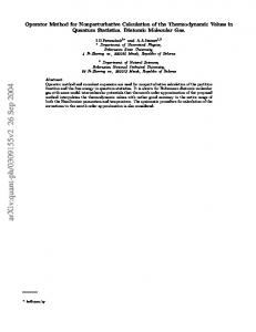
Introduction 1.1 Unsteadiness in turbomachinery There are four principal sources of unsteadiness in a single stage of a turbomachine in which there is one row of stationary blades (stators) and one row of moving blades (rotors). As shown in Fig. 1.1, wake/rotor interaction causes unsteadiness because the stator wakes, which one can consider to be approximately steady in the stator frame of reference, are unsteady in the rotor frame of reference since the rotor is moving through the wakes and chopping them into pieces. This causes unsteady forces on the rotor blades and generates unsteady pressure waves. Although the stator wakes are generated by viscosity, the subsequent interaction with the rotor blades is primarily an inviscid process and so can be modelled by the inviscid equations of motion. This allows two dierent approaches in numerical modelling. The rst is to perform a full unsteady Navier-Stokes calculation of the stator and rotor blades. The second is to perform an unsteady inviscid calculation for just the rotor blade row, with the wakes being somehow speci ed as unsteady in ow boundary conditions. This latter approach is computationally much more ecient, but assumes that one is not concerned about the unsteady heat transfer and other viscous eects on the rotor blades. Potential stator/rotor interaction causes unsteadiness due to the fact that the pressure in the region between the stator and rotor blade rows can be decomposed approximately into a part that is steady and uniform, a part that is non-uniform but steady in the rotor frame (due to the lift on the rotor blades) and a part that is non-uniform but steady in the stator frame (due to the lift on the stator blades). As the rotor blades move, the stator trailing edges experience an unsteady pressure due to the non-uniform 1

wake/rotor

interaction









HHHH Y j









utter

HHHH Y j

6

V vortex shedding

potential interaction

Figure 1.1: Sources of unsteadiness in turbomachinery ow part that is locked to the rotors, and the rotor leading edges experience an unsteady pressure due to the non-uniform part that is locked to the stators. This is a purely inviscid interaction which is why it is labelled a \potential" interaction. There are again two approaches to modelling this interaction. The rst is an unsteady, inviscid calculation of the stator and rotor blade rows. The second is an unsteady, inviscid calculation of just one of the blade rows, either the stator or the rotor, with the unsteady pressure being speci ed as a boundary condition. The latter approach is more ecient, but unfortunately the situation in which the potential stator/rotor interaction becomes important is when the spacing between the stator and rotor rows is extremely small, and/or there are shock waves moving in the region between them. Consequently, one does not usually know what values to specify as unsteady boundary conditions. The rst two sources of unsteadiness were both due to the relative motion of the stator and rotor rows. The remaining two sources are not. The viscous ow past a blunt turbine trailing edge results in vortex shedding, very similar to the Karman vortex street shed behind a cylinder. In fact real wakes lie somewhere between the two idealized limits of a Karman vortex street and a turbulent wake with steady mean velocity pro le. It is believed that provided the integrated loss is identical the choice of model does not aect the subsequent interaction with the downstream rotor blade row. However, this is an assumption which needs to be investigated sometime in the future. The importance of vortex shedding lies in the calculation of the average pressure around the blunt trailing edge, which determines the base pressure loss, a signi cant component of the overall loss. There is also experimental evidence to suggest that the vortex shedding can be 2

greatly ampli ed under some conditions by the potential stator/rotor interaction. Finally, there can be unsteadiness due to the motion of the stator or rotor blades. The primary concern here is the avoidance of utter. This is a condition in which a small oscillation of the blade produces an unsteady force and moment on the blade which due to its phase relationship to the motion does work on the blade and so increases the amplitude of the blade's unsteady motion. This can rapidly lead to very large amplitude blade vibrations, and ultimately blade failure.

1.2 A brief review In the last eight years considerable eort has been devoted to the calculation of unsteady

ow in turbomachinery. The rst signi cant piece of work was by Erdos in 1977 [9]. In his paper he presented a calculation of unsteady ow in a fan stage, including the use of an algorithm to treat unequal pitches. Unfortunately, this method has some limitations which will be discussed later. In 1985, Koya extended Erdos' work to three dimensions [21]. In 1984, Hodson modi ed a program written by Denton, and used Erdos' technique, to calculate wake/rotor interactions in a low speed turbine [18]. The incoming wakes were speci ed as unsteady boundary conditions. The results show that the wake segments cut by the turbine rotors roll up into two counter-rotating passage vortices, and the wake uid migrates to the suction surface. In 1985, Rai presented a paper showing stator/rotor interaction calculated using a Navier-Stokes algorithm [29]. This paper generated considerable interest and sparked a lot of research activity. In 1988, Rai extended his techniques to three-dimensional, viscous calculations [30]. However, Rai, along with many other researchers since, assumed that the stator/rotor pitch ratio is 1:1 or some simple ratio such as 2:3 or 3:4. This assumption allows them to perform calculations with simple periodic boundary conditions, but requires modi cations to the geometry when applied to real turbomachinery stages. In the last few years there have been several papers: Fourmaux [10] and Lewis [22], inviscid, two-dimensional stator/rotor interaction; Jorgensen [20] viscous, quasi-threedimensional stator/rotor interaction; Ni [27], inviscid three-dimensional stator/rotor interaction; Chen [4], three-dimensional, viscous stator/rotor interaction. In general, these papers have concentrated on numerical algorithm issues, and proof-of-concept demonstrations. Progressively now, the emphasis is turning to applications and mathe3

matical modelling issues such as transition and turbulence modelling. Notable work in this latter category has been done by Sharma [34].

1.3 Overview of UNSFLO and report The computer program UNSFLO which has been developed over the last ve years has many capabilities. It can solve the steady or unsteady, inviscid or viscous equations of motion in two dimensions, with extensions to include quasi-three-dimensional eects. It can handle many dierent kinds of ow unsteadiness; wake/rotor and potential/rotor interactions in which the unsteadiness is generated by unsteady in ow or out ow boundary conditions; stator/rotor interactions in which a full stage is calculated and the unsteadiness is caused by the relative motion of the stators and rotors; utter, in which the unsteadiness is due to blade vibration. One novel feature of UNSFLO is its ability to treat arbitrary wake/rotor and stator/rotor pitch ratios, which in extreme cases requires the computation to be performed on multiple rotor passages. Another is the incorporation of highly accurate non-re ecting boundary conditions which minimize non-physical re ections at in ow and out ow boundaries. A third feature is the use of unstructured grids which, in combination with an advancing front grid generator [24], makes it possible to perform calculations on complex geometries, such as pylon/strut/outlet-guide-vane combinations. Several papers have been written about dierent algorithmic components of UNSFLO, as well as the use of UNSFLO to investigate various unsteady ows. On the algorithm side the papers present the `time-inclined' computational planes used to handle arbitrary stator/rotor pitch ratios [12]; the use of \time-inclined" computational planes for convergence acceleration [11, 6]; the stator/rotor interface treatment for a transonic interaction analysis [15]; the mathematical theory behind non-re ecting boundary conditions [14]. On the application side, UNSFLO has been used to look at compressor interaction [8]; shock propagation in a shock-wave/rotor interaction [19]; complex steady and unsteady pylon/strut/outlet-guide-vane ows [24]; unsteady heat transfer in a transonic turbine stator/rotor interaction [1]. There is also a comprehensive validation paper with a number of unsteady test cases [16]. This report describes in detail the numerical method used in UNSFLO. Chapter 2 derives the explicit, Lax-Wendro algorithm which is used to calculate the unsteady, inviscid ow. It also discusses the use of an unstructured, pointered grid system, and the formulation of the numerical smoothing which is critical to the accuracy of the 4

method. Chapter 3 introduces the concept of \time-inclined" computational planes to handle unsteady calculations with arbitrary stator/rotor pitch ratios. Full details are presented on how this changes the basic Lax-Wendro algorithm. Chapter 4 shows how stator/rotor calculations are performed by calculating on two separate stator and rotor grids using relative ow variables. The two are coupled together through an interface region with moving cells. Chapter 5 presents the steady in ow and out ow boundary conditions, using non-re ecting boundary condition theory to achieve accurate results on very small domains. Chapter 6 gives the unsteady boundary conditions, which allow for the speci cation of incoming wakes and potential disturbances, and again use the non-re ecting theory to prevent arti cial re ections of outgoing waves. Finally, Chapter 7 presents the viscous ow algorithm and full details on how it is coupled to the external inviscid ow calculation.

5

Chapter 2

Lax-Wendro Algorithm on Unstructured Meshes 2.1 Unsteady Euler equations The unsteady Euler equations, describing the motion of an inviscid, compressible gas in two dimensions, are @U =  @F + @G  ; (2.1) @t @x @y where U , F and G are four component vectors given by,

1 0 1 0 0 1 v u  CC BB BB 2 CC BB CC uv u +p C u C B B C B U =B B@ v CCA ; F = BB@ uv CCA ; G = BB@ v2 + p CCA : uH

E

(2.2)

vH

The pressure p, and total enthalpy H , are related to the density , velocity components u and v , and total energy per unit mass E by the following two equations which assume a perfect gas with a constant speci c heat ratio .   p = ( 1)  E 21 (u2 + v 2) (2.3) (2.4) H = E + p : Additional equations which will be required are the de nitions of the speed of sound, Mach number, stagnation pressure and stagnation density.

c =

r p

(2.5)



6

p2 2 M = u c+ v  1  =( 1) po = p 1 + 2 M 2  1=( 1) o =  1 + 2 1 M 2 :

(2.6) (2.7) (2.8)

The ow variables are non-dimensionalized using the upstream stagnation density and stagnation speed of sound which leaves the equations unchanged and gives the following inlet stagnation quantities. (2.9) H = 1 1 ; o = 1; po = 1 : An extremely useful extension to the two-dimensional Euler equations, is the inclusion of a varying streamtube thickness in the third dimension. The resultant quasithree-dimensional equations are

where

 @(hF ) @(hG)  @U h @t = @x + @y + S; 0 BB 0@h S=B BB pp @x @ @h @y

1 CC CC ; CA

(2.10)

(2.11)

0 and h is the streamtube thickness which in general varies only in the axial x-direction. This is the most important three-dimensional eect in axial turbomachinery, but in radial turbomachinery the radius change is also very important and one should include Coriolis and centrifugal body forces [5]. These equations also apply in a rotating frame of reference at constant radius if relative velocities, total energy and total enthalpy are used.

2.2 Unstructured meshes Before beginning to present the numerical algorithm used to solve the unsteady Euler equations, it is necessary to rst discuss the organization of the computational data. Historically, most algorithms and programs in computational uid dynamics have been developed on structured meshes, which means that the computational grid is usually 7

composed of quadrilateral cells which are arranged in a logically rectangular manner and so each grid coordinate has an (i; j ) index. Each ow variable is then de ned at a particular point in a two-dimensional array, and neighboring points in the array structure are also neighboring points in the physical computational domain. The alternative approach of using unstructured meshes, is the one which has commonly been adopted in structural and thermal nite element analysis. Increasingly this approach is also being used in computational uid dynamics [25], and it is the approach used here with UNSFLO. Each grid coordinate (and its associated ow variables) is associated with a particular index in a one-dimensional array. There are also onedimensional arrays of cell-related variables, with one set of cell variables being pointers given the indices of the grid nodes which form the corners of the cell. As will be described in the next section, the ow algorithm is arranged to be implemented in a cell-by-cell manner, sweeping through the list of cells gathering the values from their corner nodes performing the necessary calculations and then distributing the appropriate changes in the ow variables back to the corner nodes. There are several reasons for choosing to use unstructured meshes. They oer great

exibility in grid generation for complex geometries, and eectively separate the process of grid generation from the ow solver, since any structured mesh can always be turned into an unstructured mesh. For added exibility, the mesh used in UNSFLO can be a mixture of quadrilateral and triangular cells. Another related advantage lies in the technique of adaptive meshes in which grids are locally re ned through the addition of extra grid points to resolve high-gradient features such as shocks and slip surfaces. This is relatively easily done for unstructured meshes [25, 7], but can only be done in a very limited and inecient way on structured meshes. Proponents and opponents of unstructured meshes disagree on both the relative ease of programming and the vector/parallel eciency of the ow solvers. The rst depends on the complexity of the geometry, since structured programs are simple for ducts, but get extremely complicated when dealing with entire aircraft, whereas the unstructured ow solvers do not change. The second point depends on the trade-o between the cost of gather/scatter operations required to address the ow variables at the corners of the computational cells, versus the increased eciency of DO-loops which span the total number of cells rather than the number in any one particular direction. The only drawback of unstructured meshes is that they are generally unsuitable in applications where ADI algorithm are required, since those algorithms require connection lists of nodes along implicit inversion lines. Even in this case, however, it is possible to construct an appropriate partially structured mesh [28]. 8

5

B

6

C 7

4

A

d

c

b

e

1

a

f

g

h

8

3

2

D 9

Figure 2.1: Control volume for quadrilateral Lax-Wendro scheme

2.3 Quadrilateral Lax-Wendro algorithm The quadrilateral Lax-Wendro scheme is very similar to that used by Ni [26] and Hall [17], but diers in precise detail for non-uniform grids. The algorithm will rst be described for the two-dimensional Euler equations, and then the modi ed version for the quasi-three-dimensional equations will be given. The second-order Taylor series expansion for U n+1 = U ((n + 1)
t) can be written as, !  @U n 2U n @ n +1 n 2 1 U = U +
t @t + 2
t @t2 : (2.12) Substituting from Eq. (2.1) and changing the order of dierentiation yields, n  @F @G n
t  @ @ n +1 n
F +
G ; (2.13) U = U
t @x + @y 2 @x @y where (2.14)
F n =
t @F ;
Gn =
t @G :

@t

@t

Now consider the cells shown in Fig. 2.1. The grid nodes are numbered, and the letters correspond to other points which will be used in explaining the method. a,c,e,g are located at the center of their respective faces, and b,d,f,h are located at the center of 9

their respective cells. Integrating Eq. (2.13) over the cell a-b-c-d-e-f-g-h-a, and applying Green's theorem, gives  I I
t 1 (2.15) (F dy G dx) + (
F dy
G dx) : U = 1

2

A1

The rst term can be split into four separate contour integrals around 1-a-b-c-1 etc., and each of these can be approximated as a quarter of the contour integral around the larger cells 1-2-3-4-1 etc., which are labelled A,B,C,D for convenience. In this manner U1 can be split into four parts,

U1 = U1A + U1B + U1C + U1D where,

U1A = A1 1


t I

4 cellA

(F dy

Z G dx)
2t

a b c

(
F dy

(2.16)
G dx)



= 4A1 (AA
UA
t (
FA (y4 y2 )
GA (x4 x2 ))) (2.17) 1 and the other terms are de ned similarly.
UA is obtained by a simple trapezoidal integration around cell A. De ning the following face lengths in a counterclockwise direction,
x21
x32
x43
x14

= = = =

x2 x3 x4 x1

x1 x2 x3 x4


y21
y32
y43
y14

= = = =

y2 y3 y4 y1

y1 y2 y3 y4

(2.18)

(2.19)

the equation for
UA is


UA =
t 21 (F1 + F2 )
y21 + 12 (G1 + G2 )
x21 AA 1 1 2 (F2 + F3 )
y32 + 2 (G2 + G3 )
x32 1 (F + F )
y + 1 (G + G )
x 4 43 2 3 4 43 2 3  1 (F + F )
y + 1 (G + G )
x : 1 14 2 4 1 14 2 4 10

(2.20)

The cell area AA is obtained from AA = 21 ( (x3 x1 )(y4 y2 ) (x4 x2 )(y3 y1 ) ) ; (2.21) and the area A1 associated with node 1 is simply an average of the four cells AA ,AB ,AC and AD .
FA and
GA are obtained from

 @F 

 @G 


FA = @U
UA ;
GA = @U
UA ; (2.22) A A with the Jacobians being evaluated using UA , the cell average of the four nodes. For computational eciency it is best not to actually form the Jacobian matrix and perform the matrix-vector multiplication. Instead, the following equations are used.
u = (
(u) u
)=
v = (
(v ) v
)=  
p = ( 1)
(E ) u
(u) v
(v ) + 12 (u2 + v 2)

F1
F2
F3
F4

= = = =


(u) u
(u) + u
u +
p u
(v) + v
u u(
(E) +
p) + H
u


G1
G2
G3
G4

= = = =


(v ) v
(u) + u
v v
(v) + v
v +
p v (
(E) +
p) + H
v:

(2.23)

(2.24)

(2.25)

By construction, the Lax-Wendro scheme as formulated here is ideally suited for calculations on an unstructured grid. In the program the algorithm is accomplished in three passes. The rst pass calculates F and G at all nodes. The second pass calculates for each cell the
U;
F;
G and then the contributions to the changes at each of its nodes. The third pass adds the changes onto the ow variables at each node and evaluates the convergence checks. The algorithm is also very suitable for calculations on a computer with either vector pipelines or multi-processors. In this case the middle pass is split into several passes. 11

The cells are \colored" such that there are no two cells of the same color touching. Then each pass calculates the update contributions from one color of cell. In this manner there are no con icts from two cells sending their contributions to the same node at the same time. The coloring algorithm need not be too sophisticated. If there are 10,000 cells then using ten colors is not much less ecient than using four. Several modi cations are needed to convert the basic two-dimensional algorithm into the quasi-three-dimensional form. The rst is that all cell areas become volumes.

A0A = 81 (h1 + h2 + h3 + h4) ( (x3 x1)(y4 y2 ) (x4 x2 )(y3 y1) ) :

(2.26)

It is also helpful to de ne the following face area terms.
x021
x032
x043
x014

= = = =

1 2 (h1 + h2 )
x21 1 2 (h2 + h3 )
x32 1 2 (h3 + h4 )
x43 1 2 (h4 + h1 )
x14

0
y21 0
y32 0
y43 0
y14

= = = =

1 2 (h1 + h2 )
y21 1 2 (h2 + h3 )
y32 1 2 (h3 + h4 )
y43 1 2 (h4 + h1 )
y14

(2.27)

(2.28)


x0024 =
x0031 =

1 (
x0 +
x0 21 14 2 1 (
x0 +
x0 32 21 2


x043
x032)
x014
x043)

(2.29)

00 =
y24 00 =
y31

0 0 1 2 (
y21 +
y14 1 (
y 0 +
y 0 32 21 2

0
y 0 )
y43 32 0 0 ):
y14
y43

(2.30)

Next, in the de nition of
UA , there are two changes, one due to the multiplication of the uxes F and G by the average streamtube thickness at the centers of the faces, and the other due to the inclusion of the source term S . This latter term can be approximated as

0 1 0 Z Z BBB @h C ZZ C @x C Sdx dy  pA B C B@ @h C dx dy @y A 0

12

0 1 0 BB H CC h dy B C = pA B B@ H h dx CCA 0

1 0 0 BB 0 +
y 0 +
y 0 +
y 0 C C
y21 B 32 43 14 C 1  4 (p1 +p2 +p3 +p4) B B@ (
x021 +
x032 +
x043 +
x014) CCA : (2.31) 0

Inserting these two changes into the ux residual equation (2.20) gives, after some tedious algebra,

1 0^ ^2 2 + V^33 + V^44 V  + V 1 1 B C B 00 (p4 p2)
y 00 C ^1(u)1 + V^2(u)2 + V^3(u)3 + V^4 (u)4 (p3 p1)
y24 V
t B 31C
UA = 2A0 B C AB @V^1(v)1 + V^2(v)2 + V^3(v)3 + V^4(v)4 + (p3 p1)
x0024 + (p4 p2)
x0031CA V^1(H )1 + V^2(H )2 + V^3(H )3 + V^4(H )4

where the V^ terms are volume uxes de ned by

V^1 V^2 V^3 V^4

= = = =

0 +
y 0 ) u1(
y21 14 0 0 ) u2(
y32 +
y21 0 +
y 0 ) u3(
y43 32 0 0 ) u4(
y14 +
y43

v1(
x021 +
x014) v2(
x032 +
x021) v3(
x043 +
x032) v4(
x014 +
x043):

(2.32)

(2.33)


F and
G are calculated in exactly the same manner as before, but the second order ux terms are slightly modi ed, so that the distributed changes to the nodes are 
t    A0   00 00 1 1 1 U1A = A0 4
t A
UA + 4
FA
y24 4
GA
x24 1   t    A0  00 00 1 1 1
F
y
G
x
U + U2A =
A A 4 A 31 4 31 4 0 
At 2  
A0t A  00 1 00 1 1 U3A = A0 (2.34) 4
t
UA 4
FA
y24 + 4
GA
x24 3 A  t    A0   1 1
F
y 00 + 1
G
x00 : U4A =

U A A A 31 4 31 4
t 4 A0 4

A

Note the rearrangement of the
t terms. Expressed in this way the numerical scheme remains conservative for steady-state calculations which use spatially varying timesteps to achieve faster convergence. 13

J

B

C JJ dH cH

A JJ

f eJJ

Hb JJ J

J J g 1J J

a

5 JJ 2 J Hh Hi

JJkJ l

JJ D

Hj J F

JJ

E JJ

6 J 7 J J

4

JJ

3

JJ

Figure 2.2: Control volume for triangular Lax-Wendro scheme

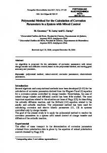
2.4 Triangular Lax-Wendro algorithm The quadrilateral Lax-Wendro algorithm has been extended by Lindquist [23] for triangular cells. The algorithm is very similar to the quadrilateral method. Fig. 2.2 shows the triangular control volume for a situation in which six triangles meet at node 1. a,c,e,g,i,k are located at the center of their respective faces and b,d,f,h, j,l are at the centers of their respective triangular cells. The counter-clockwise lengths of the faces of cell A are de ned by
x21 = x2 x1
x32 = x3 x2
x13 = x1 x3

(2.35)


y21 = y2 y1
y32 = y3 y2
y13 = y1 y3 :

(2.36)

The volume and face areas of cell A are de ned by

A0A = 61 (h1 + h2 + h3) (
x21
y32
x32
y21) ;

(2.37)

and
x021 =
x032 =
x013 =

1 2 (h1 + h2 )
x21 1 2 (h2 + h3 )
x32 1 2 (h3 + h1 )
x13

14

(2.38)

0 =
y21 0 =
y32 0 =
y13

1 2 (h1 + h2 )
y21 1 2 (h2 + h3 )
y32 1 2 (h3 + h1 )
y13

(2.39)


x0012 =
x0023 =
x0031 =


x021 + 13 (
x021 +
x032 +
x013)
x032 + 31 (
x021 +
x032 +
x013)
x013 + 31 (
x021 +
x032 +
x013)

(2.40)

00 =
y12 00 =
y23 00 =
y31

0 + 1 (
y 0 +
y 0 +
y 0 )
y21 21 32 13 3 0 0 0 0 ) 1
y32 + 3 (
y21 +
y32 +
y13 0 + 1 (
y 0 +
y 0 +
y 0 ):
y13 21 32 13 3

(2.41)

The change
UA in cell A is given by

0^ ^ ^ BB V^11 + V2^2 + V33 ^ 00 00 00
UA = 2
At B BB V^1(u)1 + V^2(u)2 + V^3(u)3 + p1
y0023 + p2
y0031 + p3
y1200 A @ V1 (v )1 + V2 (v )2 + V3 (v )3 p1
x23 p2
x31 p3
x12 V^1 (H )1 + V^2(H )2 + V^3(H )3

where the V^ terms are volume uxes de ned by 0 +
y 0 ) v1(
x0 +
x0 ) V^1 = u1 (
y21 13 21 13 0 0 0 0 V^2 = u2(
y32 +
y21) v2(
x32 +
x21) 0 +
y 0 ) v3(
x0 +
x0 ): V^3 = u3(
y13 32 13 32

1 CC CC CA (2.42)

(2.43)


F and
G are calculated as before, but the rst order term in the distributed changes is slightly dierent since the ux residual has to be distributed in equal thirds to the three corner nodes, and the second order term is dierent because of the geometric dierences between quadrilaterals and triangles. 
t    A0   00 00 1 1 1 U1A = A0
UA + 4
FA
y23 4
GA
x23 3 
t 1  
A0t A  00 00 1 1 1 U2A = A0 (2.44) 3
t
UA + 4
FA
y31 4
GA
x31 2 A  t    A0   00 1 1
G
x00 : 1 U3A =

U +
F
y A0 3 3
t A A 4 A 12 4 A 12 15

5

6

B

4

1

A

3

J

4

JJ

B

J

3 J J

CJJJ  H H

HA JJJ



J2 J



1 J

5

J

2

Figure 2.3: Cells at a wall

2.5 Wall boundary conditions At solid walls the analytic boundary condition is that there is no ow normal to the wall. Computationally this is implemented easily by setting to zero the mass ux through wall faces when calculating the change
U in any cell which has a solid wall face. To maintain vector eciency, the node-numbering of cells with wall faces is altered if necessary to ensure that the wall face is the face between nodes 1 and 2. Also the cell-coloring algorithm discussed earlier is modi ed to ensure that all cells of a particular color either do have wall faces, or do not have wall faces. Then, when looping over cells of a color with wall faces, the de nitions of the volume uxes V^1 and V^2 are changed to 0 v1
x0 V^1 = u1
y14 14 0 v2
x0 V^2 = u2
y32 32

(2.45)

0 v1
x0 V^1 = u1
y13 13 0 v2
x0 V^2 = u2
y32 32

(2.46)

for quadrilateral cells, and

for triangular cells. In addition to setting the normal mass ux to zero in the residual evaluation, at the end of each timestep the velocity is also made tangent to the wall at each surface grid node by eliminating the component of the momentum normal to the surface.

16

2 C

D

A

B 1

Figure 2.4: Grid nodes in periodic boundary condition

2.6 Periodic boundary condition The periodic condition for steady ows, and unsteady ows with equal stator and rotor pitches, is implemented by adding the update contributions that one periodic node 1 obtains from its contributing cells A and B, see Figure 2.4, to the contributions that the corresponding upper periodic node 2 obtains from its cells C and D, and using the sum to update the ow variables at 1 and 2.

2.7 Numerical smoothing Two types of numerical smoothing are added to the basic Lax-Wendro algorithm. To stabilize shock calculations and prevent large overshoots a carefully tailored seconddierence shock smoothing is used. Also, unwanted high-frequency waves in smooth

ow regions are suppressed by adding a form of fourth-dierence damping.

2.7.1 Shock smoothing The shock smoothing is similar to the second dierence smoothing used by Ni [26], but with an adaptive smoothing coecent based upon an idea of von Neumann and Richtmeyer [31]. The internal structure of a physical shock is determined by the balance of the inviscid ux and the ux due to the bulk viscosity of the uid. Thus von Neumann and 17

Richtmeyer suggested modifying the Euler equations, Eq. (2.1), into the following form, @U =  @(F F v ) + @(G G v )  ; (2.47)

@t

where F v and Gv are

@x

@y

1 1 0 0 0 0 CC CC B BB B  r :~ u 0 C CC : B B Fv = B CC ; Gv = BB B @ 0 A @ r:~u CA 0

(2.48)

0

The shock width is proportional to the bulk viscosity  divided by the magnitude of the velocity jump across the shock, and so they proposed the following formula for .

8 < 2  = : l jr:~uj ; r:~u < 0 0 ; r:~u > 0

(2.49)

Making the viscosity zero when the ow divergence is positive prevents smoothing of expansion regions. The variable l is the desired shock width which is chosen to be proportional to the local mesh spacing. The shock smoothing in UNSFLO starts with Ni's second dierence smoothing, which can be written as an additional distribution from each cell to its corner nodes. Using the same labelling system as the description of the basic algorithm, the additional smoothing distribution to node 1 due to cell A is 
t   A  [(U )1A]smoothing =  A (U1 UA ): (2.50) 1
t A In this equation UA is the average value of U in cell A, de ned by a simple arithmetic average of the nodal values. If  was taken to have a small, positive, uniform value, then this smoothing would be very similar to Ni's smoothing as described in his original paper [26]. However, in UNSFLO it is de ned to depend upon the ow divergence in a manner based on the idea of von Neumann and Richtmeyer. Firstly, a scaled ow divergence in cell A is de ned by div(~u) = (u1 u3)
y24 (v1 pv3 )
x24 + (u2 u4 )
y31 (v2 v4 )
x31 (2.51) c
x24
y31
x31
y24 for quadrilateral cells, and + u2
y31 v2
x31 + u3
y12 v3
x12 (2.52) div(~u) = u1
y23 v1
x23 p c
x12
y23
x23
y12 18

for triangular cells. These de nitions mean that in smooth regions div(~u) is approximately the ow divergence multiplied by a cell length, and in regions with a discontinuity due to a shock it is approximately the velocity jump across the shock. Next,  is de ned by







 = min 0:02; max  (2);

0:1M 2div(~u); 0:1M 2(div(~u) 0:2); 0:02(M 2 2) (2.53) The dierent terms in the above de nition require explanantion. The rst term sets an upper limit on the magnitude of ; this is needed to prevent a numerical parabolic instability. The second term is a constant which is usually zero, but can be set by the user to be a small positive constant, in which case it acts like Ni's xed-coecient smoothing. This is usually done only when there is some diculty in performing the computation without this smoothing, which might happen if there is some excessively strong ow transient. The third term is the regular bulk viscosity term which is positive only when the ow is decelerating and the divergence is negative. The Mach number is used to prevent excessive smoothing at stagnation points. The fourth term is designed to prevent the possibility of expansion shocks. It is positive only when the ow is accelerating strongly, and in almost all computations this term will be zero throughout the ow eld. The nal term introduces smoothing when the local Mach number exceeds p 2, which is above the values to be expected in most turbomachinery calculations. This term is included to cope with particular nasty transients in steady-state calculations without having to resort to a non-zero value for  (2) . It should be clear to the reader that there is a great deal of empiricism and practical experience built into the above shock smoothing formulation. All of the constants have evolved over four years of calculations, and the values above work for a wide variety of steady and unsteady turbomachinery ows. One nal important observation is that in smooth ow regions div(~u) is proportional to the local cell dimension and so if  (2) is p zero and the Mach number is below 2, then the shock smoothing is second order in magnitude and does not alter the global order of accuracy.

2.7.2 Fourth dierence smoothing Conceptually, the fourth dierence smoothing corresponds to adding a term of the form

  r: lr(l2r2U )

to the right-hand-side of Eq. (2.1) or Eq. (2.10). The variable l is a length which is comparable to the local cell length, and so the error produced by this smoothing will be 19

second-order at worst. As stated earlier, the function of this smoothing is to suppress certain highly oscillatory steady-state modes which are otherwise allowed by the basic Lax-Wendro scheme. The rst step in formulating the fourth dierence smoothing is to calculate a discrete approximation to a Laplacian of the state vector U at each node. The average gradients of U in a triangular cell can be found by an application of Green's theorem.  @U  I U dy = 1

@x

A

 @U  @y

by

A

AA

= =

cellA

1 2A (U1
y32 + U2
y13 + U3
y21) A

1 I

AA

cellA

(2.54)

U dx

= 2A1 (U1
x32 + U2
x13 + U3
x21 ): A

(2.55)

Having obtained the cell gradients, a second dierence of U at node 1 can be de ned (D2U )1  2A1 r2U1  2

 I  @U @U @x dy @y dx :

(2.56)

The line integral is around the same control volume used to assemble the second order

ux terms in the Lax-Wendro algorithm. In fully discrete form (D2U )1 is composed of contributions from all of the cells bordering node 1, and the contribution from cell A (as de ned in Fig. 2.2) is (D2U )1A = 2A1 ( (U1
y32 + U2
y13 + U3
y21 )
y32 + A (U1
x32 + U2
x13 + U3
x21)
x32 ) (2.57) Similarly the contributions from cell A to D2U at nodes 2 and 3 are (D2U )2A = 2A1 ( (U1
y32 + U2
y13 + U3
y21)
y13 + A (U1
x32 + U2
x13 + U3
x21)
x13 ) :

(2.58)

1 ( (U
y + U
y + U
y )
y + 1 32 2 13 3 21 21 2AA (U1
x32 + U2
x13 + U3
x21)
x21 ) :

(2.59)

(D2U )3A =

A noteworthy feature of this second dierence operator D2 is that when applied to a linear function U on an irregular grid, it returns a value of zero. The proof is 20

4 1

4 1

r r r @I@ r @ A4

r@ r @  @r r

3

4

4

r@ @ r @r A1

1

r

A3

3

@ cell A @ @ @

2

@

@

r

2 1

r r r

@@R

A2

3 2

3 2

Figure 2.5: Division of quadrilateral cell into triangles simple: if U is linear then rU must be uniform and so the line integral of the gradients around the node's control volume must give zero. For this to remain true at solid wall boundaries, the distribution formulae must be modi ed to include the contribution due to the control volume face lying on the wall surface. For example, in the case of cell A in Fig. 2.3, the modi ed distributions to nodes 1 and 2 are (D2U )1A = 2A1 ( (U1
y32 + U2
y13 + U3
y21 )
y13 + A (U1
x32 + U2
x13 + U3
x21)
x13 ) : (2.60) (D2U )2A = 2A1 ( (U1
y32 + U2
y13 + U3
y21 )
y32 + A (U1
x32 + U2
x13 + U3
x21)
x32 ) :

(2.61)

The discussion so far has been for triangular cells. The natural extension to quadrilateral cells would involve computing the ux of rU in each cell through the usual control volume. However, this leads to a very poor smoothing operator because an odd-even sawtooth error mode (positive at nodes 1 and 3, and negative at nodes 2 and 4) would give a rU at the cell center which is zero. Thus this error mode would not be suppressed by the smoothing. 21

Instead, the approach for quadrilateral cells is to use the triangular algorithm by dividing each quadrilateral cell into four dierent triangles (as shown in Fig. 2.5) when calculating the distributions to each of the nodes, i.e (D2 U )1A is based upon triangle A1, (D2U )2A is based upon triangle A2, (D2U )3A is based upon triangle A3 and (D2U )4A is based upon triangle A4. In UNSFLO, the second dierence function is evaluated by a preliminary sweep over all of the cells before beginning the Lax-Wendro algorithm. The fourth dierence smoothing is then built in as part of the Lax-Wendro sweep. This part of the smoothing is very similar to the shock smoothing, except that we smooth D2 U instead of U itself. In each cell the average value of D2 U is calculated and then an extra distribution is sent to each node based upon the dierence from the average value. For node 1 in either a quadrilateral or a triangular cell this addition is   A   2U )1 (D2 U )A ; (2.62) [(U )1A ]smoothing =  (4)
At ( D 1
t A with  (4) being a smoothing coecient whose value is typically taken to be 0.001.

2.8 Timestep A conservative estimate for the maximum stable timestep in each cell is given by 2A = ju
y v
x j + cq
y 2 +
x2 + 21 21 21 21
tmax q ju
y32 v
x32j + c
y322 +
x232 + q ju
y43 v
x43j + c
y432 +
x243 + q ju
y14 v
x14j + c
y142 +
x214 (2.63) for quadrilateral cells, and 2A = ju
y v
x j + cq
y 2 +
x2 + 21 21 21 21
tmax q ju
y32 v
x32j + c
y322 +
x232 + q ju
y13 v
x13j + c
y132 +
x213 (2.64) for triangular cells. All terms are as de ned earlier in this chapter, with u; v; c based upon the cell-averaged ow quantities. For unsteady calculations the uniform global timestep is taken to be the minimum over all of the cells of the local maximum timestep, multiplied by a CFL number which is typically taken to be 0.9. 22

For steady calculations, local time steps are used to march to steady-state convergence as quickly as possible, so one used the local maximum timestep multiplied again by a CFL number which is typically 0.9. The area/timestep ratio associated with a grid node is then de ned by

A

A

X


t node = cells fcell
t cell ; where the sum is over all of the neighboring cells and fcell is and 31 for triangular cells.

(2.65) 1 4

for quadrilateral cells

2.9 Conservation In earlier sections it has been stated that the Lax-Wendro algorithm, as implemented here, is conservative in the solution of the nonlinear Euler equations. It is appropriate now to discuss what this statement means for both steady and unsteady ows, and to outline the proof of conservation for the given algorithm. Steady-state solutions of the two-dimensional Euler equations satisfy the following integral equation, evaluated by a counter-clockwise integration around the domain.

I

(F dy G dx) = 0

(2.66)

A steady, discrete solution is said to be conservative if, for any domain composed of a group of cells, there is a corresponding discrete equation which approximates this integral equation, and becomes equal to it in the limit of in nite grid resolution. The importance of conservation is due to the fact that this property guarantees the correct Rankine-Hugoniot jump relations across a shock and the correct treatment of other discontinuities such as slip lines (assuming the solution is suciently smooth away from the discontinuity). Thus conservation for nonlinear discontinuous solutions is similar to consistency for nonlinear smooth solutions as a requirement in order to obtain a discrete solution which will approach the analytic solution as the mesh is re ned. Similarly, unsteady analytic solutions satisfy the following equation.

d Z Z U dx dy + I (F dy G dx) = 0 dt

(2.67)

Discrete solutions are conservative if they satisfy an equivalent discrete solution. To prove that the Lax-Wendro scheme is conservative we must show that

X A i




t U = i

X

(boundary uxes):

23

(2.68)

The change Ui is equal to a sum of the contributions from all of the cells of which node i is a corner. The order of summation can then be interchanged to obtain

X A i



X

i

cells


t U =

(sum of contributions to corner nodes)

(2.69)

The second order inviscid ux terms and both the shock and fourth-dierence smoothing terms were written in such a way that the sum of their contributions to the corner nodes of a cell is zero. This leaves only the rst order inviscid ux terms, and hence

X A i


t U



XA




t
U i cells X (inviscid uxes out of cell) = =

cells

(2.70)

The nal step is the observation that the ux out of a particular cell across a particular face is equal and opposite to the ux out of the neighboring cell across the same face. Thus all interior uxes cancel leaving the desired result, Eq. (2.68). For quasi-three-dimensional ows the theory is modi ed slightly by the presence of the pressure source term in the momentum equations, and so the analytic and discrete conservation relations have an additional area integral/summation of the source term. The basic concept remains the same, however, and so does the proof.

24

Chapter 3

Time-Inclined Computational Planes 3.1 Lagged periodic condition When the stator/rotor pitch ratio is unity the periodic boundary condition is simply,

U (x; y; t) = U (x; y + P; t);

(3.1)

meaning that what is happening on the lower periodic line is exactly the same as is happening on the upper periodic line at exactly the same time. When the stator pitch is dierent from the rotor pitch this has to be changed. Considering the case of wake/rotor interaction, in which the stator pitch is larger than the rotor pitch, then an incoming wake (moving downwards in the rotor frame) crosses the inlet boundary/upper periodic boundary junction a small time
T after the neighboring wake crosses the inlet/lower periodic junction. Thus the inlet boundary conditions satisfy the lagged periodic condition,

U (x; y; t) = U (x; y + Pr ; t+
T );

(3.2)

where the time lag,
T , is equal to the dierence in pitches divided by the rotor wheel speed.
T = (Ps Pr )=V (3.3) The next step is to apply this lagged periodic condition to the upper and lower periodic lines. Strictly speaking this is an assumption about the nature of the ow 25

s s

6 Ps

t@ t+
T @@

 

@@@@ @@R R @

V

?

6 Pr

?

?

Figure 3.1: Origin of lagged periodic boundary condition produced by the wake rotor interaction. There are many examples in mathematics (including some fairly simple examples in dynamics) in which periodic terms (either as forcing terms or time-varying coecients) produce solutions with a subharmonic component, a component whose period is a multiple of the original period. As an example, consider vortex shedding from a turbine row. Imposition of spatially periodic boundary conditions forces the solution to exhibit synchronous shedding, in which each blade sheds vortices of the same sign at the same time. However it may be true that in actuality the blades shed at the same time, but shed vortices of alternating sign, with one blade shedding a vortex of positive sign at the same time that its two neighbors shed vortices of negative sign. This would be an example of a spatial subharmonic whose period is 2Pr . Mathematically, the spatially periodic solution produced by the program would be a valid solution to the unsteady Euler equations, but it would have a linear, subharmonic instability which would grow into the fully nonlinear, subharmonic shedding. In this case to compute the true solution would require a computational domain spanning two blade passages.

26

cHYHss HsH s s s ss ss ss: c ssHHHHHHH ss HH Hs ss s s s

6 t t
T t (T
T )

dummy node

Pr

0

y

-

Figure 3.2: Erdos' periodic boundary treatment

3.2 Erdos method Erdos [9] was the rst researcher to develop a solution to the problem of the lagged periodic boundary condition. As illustrated in Figure 3.2, his procedure involves setting values at dummy points along each periodic line from stored values at points along the other periodic line at earlier times. The value at the dummy point on the upper periodic line is obtained from the equation

U (x; y; t) = U (x; y Pr ; t
T ):

(3.4)

To obtain the value on the lower periodic line, it must be assumed that the ow is periodic in time, with period equal to the blade passing period T = Ps =V . With this assumption, it follows that

U (x; y; t) = U (x; y + Pr ; t +
T ) = U (x; y + Pr ; t (T
T ));

(3.5)

The implementation of this requires storing the full solution along the periodic lines for a whole period. This can involve a considerable amount of storage. However, the primary drawback of this method is the assumption of periodicity in time. This is probably valid only when calculating inviscid ows. In viscous ows there are physical instabilities and oscillations, such as vortex shedding at the trailing edge, in which the frequency is not a multiple of the blade-passing frequency. In these situations Erdos' method would fail to converge to a consistent periodic solution. The new computational method using inclined computational planes avoids this assumption. 27

s s    s s   s  s  6

t+
T t

Pr

0

y

-

Figure 3.3: Concept of inclined computational plane

3.3 New computational method Computationally it is very easy to enforce the spatial periodicity for steady ows, as described in an earlier section. For unsteady ows with the lagged periodicity condition it was desired to have as simple an implementation. This led to the following idea: suppose that instead of a computational \time level" being at a xed time, it is sloped in time such that if a node at y = 0 is at time t, then the corresponding periodic node at y = Pr is at time t +
T , and so once again one has simple spatial periodicity in this inclined computational plane. Fig. 3.3 illustrates this concept. Mathematically this corresponds to the following coordinate transformation.

x0 = x y0 = y   t0 = t
PT y r

(3.6)

In this new coordinate system each computational plane corresponds to t0 =constant. When one transforms the unsteady Euler equations the resultant equations are,

@ @F @G @t0 (U G) + @x0 + @y 0 = 0

(3.7)

with  =
T=Pr . Thus, the conservation state variables have changed from U to U G. An alternative way of arriving at the same conclusion is to consider the conservation cell shown in Fig. 3.4 in the original (y,t) plane. The ux through the \time-like" face is U
y G
t = (U G)
y . 28

6  6      G     U

t

          y

-

Figure 3.4: Inclined conservation cell The change in the conservation variables requires just minor changes to the LaxWendro algorithm, because fortunately one can calculate U from Q = U G in closed form for a perfect gas.

q1 =  v

(3.8)

q2 = u uv = q1 u

(3.9)

q3 = v (v2 + p) = q1 v p



q4 = 1 1 p + 12 (u2 + v 2) v 1 p + 21 (u2 + v2) 1  1 2 2 = q1 2 (u + v ) + 1 p  1 pv



(3.10)

(3.11)

Eliminating u and v using the last three equations gives a quadratic equation for p.

Ap2 2Bp + C = 0

(3.12)

A = ( +1)2 B = q1 q3 C = ( 1)(2q1q4 q22 q32 )

(3.13)

where,

This has solutions,

p=

pC 2 : B  B AC 29

(3.14)

The positive root is chosen because this gives the correct value in the limit  = 0. u; v and  are then obtained from

u = qq2 1 v = q3 +q p 1  = 1 q1v :

(3.15) (3.16) (3.17)

Eqs. (3.14)-(3.17) can also be linearized to obtain the following equations.





( 1) 21 (u2 + v 2)q1
q1 + q1
q4 q2
q2 q3
q3 + p(
q3 v
q1)
p = (1 v)2 2 p
u =
q2 q u
q1 1

(3.18)
v =
q3 v
q q1 + 
p 1
v
 =
q11 +  v The fact that the independent variable is now Q instead of U requires two changes to the basic Lax-Wendro algorithm. The ow variables that are stored are still the standard conservation variables U . These are used as before to calculate the uxes F and G, and the cell residual on both quadrilateral and triangular cells. However, these cell residuals, which before de ned the change
U , now give the change
Q. The linearized equations Eqs. (3.18)-(3.19) are then used to evaluate
F and
G in the cell. The distribution equations now give changes in Q at the nodes. For example, the equations for quadrilateral cells are 
t    A0   00 00 1 1 1 Q1A = A0 4
t
QA + 4
FA
y24 4
GA
x24 1 
t    A0 A  00 00 1 1 1 Q2A = A0
F
y
G
x
Q + A A 4 A 31 4 31 4 
t 2  
At0 A  00 00 1 1 1
Q Q3A = A0
F
y +
G
x (3.19) A 4 A A 24 4 24 4
t A 3 
t    A0   00 00 1 1 1 Q4A = A0 4
t
QA 4
FA
y31 + 4
GA
x31 4

A

The smoothing terms are handled exactly as before. The nal step is to take the old variables U n , calculate Qn , add the change Qn to obtain Qn+1 and then use Eqs. (3.14)(3.17) to convert back to U n+1 . The additional work involved in these steps is approximately 15% of the cost of the basic algorithm. 30

t

dt 1 1 dt 6dydt = c 1v dy = v dy = c+v * I@ @ 
 Q  Q
HHHQQ@@  
PPPPHHHQQ@
 ((( permissible Q @ H P
hhhhhhPhPPHPHQQ@
(((((((( computational hh(hPH(hPHQ@(HPh
(h(h(( planes  P Q ( h ( h H  P ( h ( h QQHHPPP hhhhhh (((( QQHQHHPHPPPP hh

y

Figure 3.5: Physical characteristics and permissible values of 

3.4 Multiple blade passages The need for multiple blade passages in some calculations arises from a fundamental limit on the magnitude of . Re-examining Eqs. (3.8)-(3.14), and de ning rv = v and rc = c, it can be shown that,   1 2 2 B =  (1 r ) + r (3.20)



v

C = p 2(1 r v and hence that Eq. (3.14) reduces to



)2

c

1 r2  ;

c

(3.21)



2(1 r v )2 1 rc2 p p p= (1 r v )2 + 1 rc2  ((1 r v )2 rc2)2

(3.22)

When  = 0 the positive root reduces to p, while the negative root is in nite, and so, as stated earlier, the positive root is chosen for all values of . This remains correct at non-zero values of  provided (1 rv)2 > rc2 . Assuming that the ow is subsonic in the y-direction this condition can be re-expressed as, 1 1 (3.23) c v <  < c+v As shown in Fig. 3.5 this condition means that the slope of the computational plane may be increased or decreased up to the point at which it is coincident with one of the three physical characteristics of the Euler equations. This is clearly a fundamental physical limitation because beyond this point a signal which propagates forward in time in the physical coordinates would be propagating backward in time in the computational 31

coordinates, which is clearly inconsistent with the numerical procedure which marches forward in time. Substituting the de nition of  gives the corresponding limits on the stator/rotor pitch ratio. (3.24) 1 Mr < Ps < 1 + Mr 1 M y Pr 1+ M y My = v=c is the Mach number in the y-direction, and Mr = V=c is the Mach number associated with the rotor speed V . The range of possible pitch ratios clearly depends most strongly on Mr . In most practical turbomachinery applications Mr lies in the range 0.3-0.6, allowing pitch ratios in the range 0.6-1.5. Unfortunately many detailed experiments are performed for good experimental reasons on large scale, low speed rigs for which Mr is substantially lower (0.05-0.2) producing a much smaller range of possible pitch ratios. In either case there are plenty of examples of situations in which the geometry to be analyzed lies outside the range of pitch ratios which can be analyzed by the current method as described so far. The solution to this problem is to perform calculations on multiple blade passages. If, for example, the stator/rotor pitch ratio is exactly 2.0, then this case could be calculated on a grid covering two rotor passages, without requiring any time inclination of the computational plane, i.e. with  =0. At the other extreme, if the ratio is exactly 0.5 then this case could be calculated on a single rotor passage, but with two wakes speci ed at the inlet plane. In the most general case the calculation is performed on m rotor passages, with n wakes (or potential disturbances) speci ed at the inlet (or outlet) plane. The ratio m=n is chosen to be approximately equal to the pitch ratio. If it is exactly equal then no time inclination is required. If it is not exactly equal then  \makes up the dierence" in the same way as before.  =
T = 1 n Ps m Pr

m Pr

m Pr V  P m 1 (3.25) = V Ps = n 1 r In operation, the user of UNSFLO speci es m, which controls the size of the compu-

tational grid and the corresponding computational cost, and the program calcuates the value of n which minimizes the magnitude of . Clearly the larger the value of m, the closer the fraction m=n will be to the pitch ratio Ps =Pr , and so the smaller  will be. Thus for any pitch ratio and any values of Mr and My it is possible to nd a value for m such that  will not violate the domain of dependence restrictions discussed earlier. 32

Chapter 4

Stator/Rotor Interface Region This section describes the computational algorithm used for calculations in which there are two blade rows moving relative to each other. The algorithm for the case in which the blade rows have equal pitches is presented rst, because it is relatively easy to visualize and it contains all of the essential new algorithm components. Then, the algorithm for the general case of unequal pitches is presented. This uses the timeinclined computational planes described in the last section, and viewed from a purely mathematical viewpoint it is a straightforward extension of the equal pitch method. However, it becomes extremely dicult to visualize the shearing, inclined computational cells which are involved. 1

4.1 Algorithm for equal pitches The basic geometric approach is shown in Fig. 4.1. The computational grid is composed of two parts, one part xed to the stator blade row (which in this discussion will be assumed to the upstream blade row) and the other part xed to, and moving with, the rotor blade row. The two parts are separated by a cell width at the interface, with equal grid node spacing along the interface on either side. In this section we will assume that there are the same number of grid nodes on both sides of the interface, so that the gap between the two halves can be spanned by a set of quadrilateral cells de ned by connecting each stator grid node to the nearest rotor grid node. In a later section we will present an alternative treatment with triangular cells which allows unequal number 1 In fact, in my experience trying to visualize and understand it can quickly cause a severe headache

which can only be relieved by taking a long walk!

33

Stator grid

  HHH   H   HHH   H   HHH   H 

6

V

Rotor grid

Figure 4.1: Shearing cells at unsteady stator/rotor interface 3

 2         4  A 1  

cs cs

Figure 4.2: Periodic extension of rotor grid

of nodes on either side of the interface. As time progresses, the rotor moves and the cells change from State 1 (with solid lines) to State 2 (with dotted lines) to State 3 (with dashed lines). At that time the connecting lines are rede ned to maintain nearest neighbor connections, and the cells revert to State 1. As shown in Fig. 4.2, spatial periodicity is used to extend the rotor grid as needed as the rotor grid moves. The solid lines denote the actual position of the rotor grid and the dotted lines show the position of the rotor grid shifted by one pitch. The open and closed circles denote matching pairs of rotor nodes, so that when the computation is performed on cell A, the distributions really go to nodes 1, 2, 3 and 4. On each half of the grid the ow solution is calculated using local grid-relative ow variables. This allows one to use the Lax-Wendro algorithm described in Chapter 2 without modi cation. At the interface cells the basic algorithm has to be modi ed for 34

two reasons. Firstly, all ow variables have to be converted into some chosen frame of reference and when the ow change are calculated they must be converted back into the local frame of reference. In the analysis presented, and in the implementation in UNSFLO, the chosen frame of reference is the absolute stator frame. It can be veri ed (and has been both on paper and by programming) that using another frame of reference will produce the same nal results. The rotor-relative and stator-relative ow variables are related by

s us vs ps

= = = =

r ur vr + V pr ;

(4.1)

where V is the rotor wheel speed, and the subscript s denotes stator-relative values and the subscript r denotes rotor-relative values. Hence

0 BB Ur1 Us = B BB Ur2 @ Ur 3 + V Ur 1

1 CC CC CA

0 Us1 B B Us2 Ur = B B B @ Us3 V Us1

1 CC CC ; CA

Ur4 + V Ur3 + 12 V 2Ur1

and

Us4 V Us3 + 12 V 2 Us1

0 Us1 B B Us2 Ur = B B B @ Us3 V Us1

Us4 V Us3 + 21 V 2 Us1

(4.2)

1 CC CC : CA

(4.3)

(4.4)

Eq. (4.2) is needed at the beginning of the cell calculation to convert the rotorrelative values on the rotor side of the interface into stator-relative values. Eq. (4.4) is needed at the end of the cell calculation because the ow variable changes distributed to the nodes on the rotor side of the interface are changes in stator-relative quantities that have to be converted into changes in rotor-relative quantities. 35

3

    6  4 V

1

 2    

Figure 4.3: Shearing interface cell The second modi cation to the basic Lax-Wendro algorithm is due to the movement of the computational cell. The change is best understood by considering the following integral form of the two-dimensional Euler equations on a control volume whose boundary has a unit normal vector ~n and is moving with velocity V~ = (Vx; Vy )T .

d Z Z U dx dy = Z Z @U dx dy + I U (V~ :~n)ds dt I @t I = (F dy G dx) + (UVx dy UVy dx)

(4.5)

Considering the computational cell shown in Fig. 4.3, the extra ux term across face 1-2 is approximated by treating U as being linear.

Z x2 x1

UVy dx =
x21

Z1 01

(U1 +  (U2 U1)) V d



=
x21 6 U1 + 31 U2 V

Including the corresponding term on change
UA is
UA =
t ( (F1 + F2 )
y21 2AA + (F2 + F3 )
y32 + (F3 + F4 )
y43 + (F4 + F1 )
y14

(4.6)

face 3-4, the modi ed equation for the cell (G1 + G2 )
x21 + ( 13 U1 + 32 U2 )V
x21 (G2 + G3)
x32 (G3 + G4)
x43 + ( 23 U3 + 13 U4 )V
x43 (G4 + G1)
x14 ): (4.7)

The second order terms in the distribution formulae also change because of the motion of the control volume. 
t    A   1 1 1 1 V U1A = A 4
t
UA 4
FA (y4 y2 ) + 4
GA (x4 x2 ) 4
UA 4 (x4 x2 ) 1 A 36


t    A  U2A = A 41
t
UA 
t 2   A A

1
FA (y1 4

y3) + 14
GA (x1

1
F (y 4 A 4

U4A =

1
FA (y1 4

U3A =

1 4
t A
UA + A 3 
t    A  1 A 4 4
t A
UA +

x3 )

y2 )

1
GA (x4 4

x2 ) + 14
UA 34V (x4

x2 )

y3 )

1
GA (x1 4

x3 ) + 14
UA V4 (x1

x3 ) :

x3 )

(4.8)

4.2 Algorithm for unequal pitches When the pitches of the stator and rotor are unequal, the conceptual approach remains the same, but the details become much more complicated. Time-inclined computational planes are used to calculate the ow in both the stator and rotor halves of the computational grid, but the time-step and inclination parameter  are dierent in the two halves. In the stator frame of reference the blade-passing period is

Ts = Pr =V;

(4.9)

Tr = Ps=V;

(4.10)

The calculation has the same number of time-steps per period on each half, so the time-steps on the two halves are related by
ts = Pr : (4.11)
tr Ps Similarly, the lagged period boundary condition in the stator frame is

U (x; y; t) = U (x; y + Ps ; t +
T );

(4.12)

and in the rotor frame it is

U (x; y; t) = U (x; y + Pr ; t +
T );

(4.13)

with the time lag
T given by
T = Ps V Pr = Tr Ts : 37





As explained earlier, the distributions to nodes 2 and 3 must be converted into rotor-relative changes using Eq. (4.4).

whereas in the rotor frame it is



1
UA 3V (x1 4 4

(4.14)

Consequently, the time-inclination parameters in the two frames of reference are (4.15)  =
T = Ps Pr ; s

and

Ps

V Ps

(4.16) r =
PT = PsV P Pr : r r The diering values of
t and  in the two frames of reference are extremely con-

fusing; it is hard to understand how this can be consistent at the stator/rotor interface. Fig. 4.4 attempts to explain this by showing both the stator and rotor inclined computational grids in the stator frame of reference. The gure shows a case in which the the stator pitch Ps is greater than the rotor pitch Pr , and, for simplicity, there are only six timesteps per period, and only ve cells spanning one pitch. The stator and rotor nodes are aligned so that they coincide at the beginning of a computational period. There are several important things to note in the diagram. At each time-level, the stator and rotor grids lie on the same inclined computational plane, but the rotor grid is displaced relative to the stator grid. The circles denote three points which are de ned to be equal through the lagged periodic boundary condition, and so computationally correspond to the same two points (one on the stator side of the interface, the other on the rotor side). The diagram shows that the stator node spacing
ys is greater than the rotor node spacing
yr at xed time t, but that on the inclined computational plane the rotor node spacing becomes equal to
ys . Thus, viewed on the inclined stator computational plane, the shearing cell in the interface region is a parallelogram, exactly the same as in the case of equal stator and rotor pitches. The diagram also shows that the stator timestep
ts is not equal to the rotor timestep
tr , even though both grids are consistently at the same computational time level. This is because the spatial shift of the moving rotor grid produces a temporal shift on the inclined computational grid. One nal observation is that the velocity of the rotor changes when viewed in the stator inclined computational plane. It travels one pitch Ps in an apparent time of Pr =V , the time between the rst and last time-level in a stator period, and so its apparent speed is

Vs = V PPs : r

(4.17)

Similarly, in the inclined rotor frame of reference the apparent speed is

Vr = V PPr : s

38

(4.18)

6  

Rotor periodic   nodes HH

Stator periodic nodes HH

HHH

Hj

HHj 




















t














 
















 









 











 









 








 Ps =V 




 


 




 


   




 

  6  










tr     

  
   





 
    




  Pr =V
 ? 

 




   









 

   









 

       
 









  
 



 

  6    






ts 




 
  
?









 











 





 6









Inclined





computational

 
plane 


















-

-


0 P P 2 P 2 P r s r s y
y
y

d

d

d

t

t

t

r

s

Figure 4.4: Inclined computational planes at stator/rotor interface

39

The algorithm for the interface region follows the same approach as for equal pitches. The rst step is to form a set of shearing parallelograms in the stator inclined computational plane, by connecting stator nodes to rotor nodes, using spatial periodicity as needed. The second step is to convert the rotor-relative ow variables at the rotor nodes to stator-relative ow variables using Eq. (4.2). The modi ed equation for
QA at the center of the shearing cell is similar to Eq. (4.7). However the apparent rotor speed Vs and the modi ed conservation variable Q must be used instead of V and U respectively. Also introducing the quasi-threedimensional terms gives the following equation.

1 0^ ^2 2 + V^33 + V^44 V  + V 1 1 BB ^ C 00 (p4 p2)
y 00 C V (u)1 + V^2 (u)2 + V^3(u)3 + V^4(u)4 (p3 p1)
y24
t 1 B 31C
QA = 2A0 B C AB @V^1(v)1 + V^2(v)2 + V^3(v)3 + V^4(v)4 + (p3 p1)
x0024 + (p4 p2)
x0031CA V^1(H )1 + V^2(H )2 + V^3(H )3 + V^4(H )4


t ( 1 Q + 2 Q )V
x0 + ( 2 Q + 1 Q )V
x0  2A0A 3 1 3 2 s 21 3 3 3 4 s 43

(4.19)

The geometric and V^ variables are as de ned in Chapter 2.
U ,
F and
G are calculated from
Q in the usual manner, and then the distribution formulae are  
t    A0  00 00 00 1 1 1 1 V Q1A = A0 4
t
QA + 4
FA
y24 4
GA
x24 + 4
QA 4
x24 1 A 
t    A0   00 00 00 1 1 1 3 V 1 Q2A = A0 4
t
QA + 4
FA
y31 4
GA
x31 + 4
QA 4
x31 2 A   t    A0  00 00 3V
x00 1 1 1 1
F
y +
G
x
Q Q3A =

Q A0 3 4
t A A 4 A 24 4 A 24 4 A 4 24  t    A0   00 00 00 1 1 V 1 1 Q4A =

F
y +
G
x
Q
x
Q A0 4 4
t A A 4 A 31 4 A 31 4 A 4 31 : (4.20) s

s

s

s

The smoothing terms are calculated and distributed as normal. The nal step is the conversion of the distributed changes to nodes 2 and 3 from stator-relative changes to rotor-relative changes. There are two components to this. One is due to the dierent
t and
y in the two frames of reference (as discussed earlier).

A

 P 2  A  r


t r = Ps 40


t s :

(4.21)

The other is similar to the conversion from Us to Ur , except that the conversion is now from Qs to Qr , making the algebra considerably more complicated although the nal result is almost identical.

0 BB  v Qr = B BB u uv2 @ v (v +p)

E (E + p)v

1 CC CC CA

rotor

1 Ps Pr v CC VP CC Ps r Pr uv C VP CC Ps rPr (v2 + p) C CC V Pr A P P s r E V P (E + p)v r rotor 1 0 Pr Ps Pr CC B Ps  V Ps (v V ) B CC B Pr u Ps Pr u(v V ) B CC B Ps V Ps = Ps B CC B Pr (v V ) Ps Pr ((v V )2 + p) Pr B CC B V Ps B @ PPsr 1 V 2 ) Ps Pr ((E vV + 1 V 2)+ p)(v V )) A  ( E vV + 2 2 Ps V Ps stator 1 0 Ps Pr  V P v CC B s B CC B Ps Pr uv B u CC B V Ps = Ps B CC B Pr B (v V ) PsV P Pr (v(v V )+ p) CC B B s A @ (E vV + 12 V 2 ) PsV P Pr ((E vV + 21 V 2 )+ p)v pV ) s stator

0 BB  BB B u = B BB BB v @

0  v B B u uv = PPs B B B r @ (v V ) (v (v V )+ p)

(E vV + 12 V 2 ) ((E vV + 21 V 2)+ p)v pV )

0 Q1 B B Q2 = PPs B B B r @ Q3 V Q1

Q4 V Q3 + 21 V 2 Q1

1 CC CC CA

1 CC CC CA

stator

(4.22) stator

41

Stator grid

   XXXX    ZZ   ZZ HHHH  

6

V

Rotor grid

Figure 4.5: Triangular cells at unsteady stator/rotor interface Thus, the equation to convert the distributed changes into rotor-relative changes is

0 BB Q1  A  Q2 Pr A B Q = B r
t r Ps
t s B @ Q3 V Q1

Q4 V Q3 + 12 V 2 Q1

1 CC CC : CA

(4.23)

s

4.3 Unequal numbers of interface nodes In the rst section in this chapter, an assumption was made that the number of grid nodes on either side of the stator/rotor interface is equal. This is generally desirable, but sometimes it is useful to be able to perform calculations with diering numbers of nodes on the two sides. In this case, it is no longer possible to span the interface gap with quadrilaterals. Instead, triangular cells are created in the time-inclined stator frame by joining each cell face on either side to the node on the opposing side which is closest to the face's midpoint. Fig. 4.5 shows a typical interface region created by this technique. The discrete equations for the shearing triangular cells in the interface region take diering forms depending on whether the majority of the nodes are on the stator or rotor side. If nodes 1 and 3 are on the stator side of the interface, then the cell change
QA is given by 1 0^ ^22 + V^3 3 V  + V 1 1 BB ^ C 00 + p2
y 00 + p3
y 00 C V
t 1(u)1 + V^2(u)2 + V^3(u)3 + p1
y23 B 31 12C
QA = 2A0 B C AB @V^1(v)1 + V^2(v)2 + V^3(v)3 p1
x0023 p2
x0031 p3
x0012CA V^1(H )1 + V^2(H )2 + V^3(H )3 42


t ( 1 Q 1 Q )V
x0  (4.24) 2A0A 3 1 3 3 s 21 The geometric and V^ variables are again as de ned in Chapter 2.
U ,
F and
G are calculated from
Q in the usual manner, and then the distribution formulae are 
t    A0   V s 00 00 00 1 1 1 1 Q1A = A0 2
t
QA + 4
FA
y23 4
GA
x23 + 4
QA 4
x23 1 A 
t    1
G
x00 1
F
y 00 Q = 2A

Q3A

4 A 31 A0 2 
t    A0  00 = A0 21
t
QA + 14
FA
y12 3 A

4

A

31

Vs 00 00 1 1 4
GA
x12 + 4
QA 4
x12



(4.25)

Note the fact that the rst order distribution term going to node 2 is zero, and so nodes 1 and 3 equally share the rst order changes. This was done because the only way for the scheme to remain conservative is to consider half of the triangle's area to `belong' to node 1 and the other half to node 3. This way the nodal areas of 1 and 3 remain constant because each `owns' half of the two triangles on either side. Given this apportioning of the cell area, the rst order change has to be distributed consistently. For a triangular cell with nodes 2 and 3 on the rotor side, the corresponding equations are,

1 0^ ^22 + V^3 3 V  + V 1 1 B C 00 + p2
y 00 + p3
y 00 C B ^1(u)1 + V^2(u)2 + V^3(u)3 + p1
y23 V
t B 31 12C
QA = 2A0 B C AB @V^1(v)1 + V^2(v)2 + V^3(v)3 p1
x0023 p2
x0031 p3
x0012CA V^1(H )1 + V^2(H )2 + V^3(H )3


t ( 2 Q 2A0A 3 2 and

2 Q3 )Vs
x0 21 3




t  

;

1
FA
y 00 Q1A = A0 23 4 1 
t    A0  00 Q2A = A0 12
t
QA + 14
FA
y31 2 A 
t    A0  00 Q3A = A0 12
t
QA + 14
FA
y12 3 A

43

(4.26)



00 1 4
GA
x23 00 1 1 3V 4
GA
x31 + 4
QA 4


x00

00 1 1 3V 4
GA
x12 + 4
QA 4


x00

s

s

31 12

 

(4.27)

The smoothing terms are calculated and distributed as usual. Finally, the conversion of the distributions from stator-relative changes to rotor-relative changes is exactly the same as for the quadrilateral algorithm.

4.4 Multiple blades As with wake/rotor calculations, there are situations in which stator/rotor calculations with just one stator and one rotor leads to time-inclination parameters which are too large. In this case it may be necessary to perform the calculation with m rotors and n stators. All of the preceding discussion in this chapter remains valid by considering an equivalent stator pitch which is equal to nPs and an equivalent rotor pitch which is equal to mPr . Thus, the time-tilting parameters in the stator and rotor frames are

 nPs  nPs  s = V1 mP 1 r  nPs  mPr 1 r = V mP 1 ; r

1

(4.28)

and the periods in the two frames of reference are r Ts = mP jV j s: Tr = nP jV j

44

(4.29)

Chapter 5

Steady Boundary Conditions 5.1 Overall approach This section describes the numerical in ow and out ow boundary conditions which are used for calculations of steady ow. They are an implementation of a theoretical development in non-re ecting boundary conditions which is presented in Refs. [13, 14]. The objective of non-re ecting boundary conditions for steady ows is to be able to bring the far- eld boundary location relatively close to the blades without aecting the ow eld in the neighborhood of the blades. The smaller computational domain leads to much more ecient calculations. It is also very important when doing steady stator/rotor calculations since the spacing between the blade rows can be quite small. The approach is based upon a characteristic analysis of the linearized Euler equations. At each in ow or out ow boundary there is a certain number of incoming modes and a certain number of outgoing ones. The changes in the outgoing characteristic values are taken from the changes distributed by the Lax-Wendro algorithm. The average changes in the incoming characteristics are determined to satisfy a number of user-speci ed average quantities. At the in ow these are ow angle, stagnation denity and stagnation enthalpy. At the out ow it is the average static pressure. The remaining changes, the spatial harmonics of the incoming characteristics are speci ed by the non-re ecting boundary condition theory based upon the the amplitudes of the corresponding spatial harmonics of the outgoing characteristics.

45

5.2 Average ow de nitions The computational grid is constructed so that the grid nodes are equally spaced along the in ow and out ow boundaries. The average values of any ow quantity  can be de ned by X (5.1)  = N1 j j

where the sum is over the N nodes at the boundary, including the periodic grid node only once. If the Euler equations were linear then this de nition would be all that was required. However, because of non-linearities, the average value of a variable will not in general be equal to its value based upon averages of other variables. For example,   p 6= ( 1) E 21 (u2 +v2) (5.2) Hence, this raises the question of what is the correct way in which to perform the averaging procedure. The only rigorous de nition is based upon the `mixed-out' ow eld. This approach starts from the two-dimensional Euler equations, integrated in the y -direction over one pitch.

d Z P F dy = Z P @F dy dx 0 0 @x Z P @G = @y dy 0 = G(0) G(P ) = 0

(5.3)

Thus, if one assumes that suciently far upstream or downstream the ow is uniform, then the ux F based upon this uniform value UF must be equal to the average ux F at the boundary under consideration. This gives the following set of equations for UF . F uF = F1 F uF2 + pF = F2 F uF vF = F3 (5.4) F uF HF = F4 Together with the equation

  p HF = 1 F + 12 uF2 + vF2 F 46

(5.5)

these can be solved to obtain   q 1 2 2 2 2       pF = + 1 F2 + F2 + ( 1)(F2 + F3 2F1F4 ) F p uF = 2 F F 1  vF = FF3 1  F = Fu 1

(5.6)

F

Based on these values, `mixed-out' values of all other ow variables can be de ned, and will be denoted by the subscript F . An important point to note is that the physical mixing process implied in this procedure will generate viscous losses, and will result in a ow with a higher entropy level. Hence, when applied to ow at the out ow boundary this averaging procedure will tend to produce higher `measured' losses than other averaging methods, such as averaging the outgoing entropy. The same ux-averaging method can also be used to determine losses in an unsteady

ow. In this case the ux components must be averaged in time as well as in space, over a time interval which for periodic ows is the period, and for non-periodic ows is large compared to any other time-scales in the ow.

5.3 Characteristic variables When calculating the change in the boundary values from time level n to time level n+1, the characteristic variables are de ned in terms of perturbations to the average in ow or out ow ow eld at time level n. As shown in Reference [13], the one-dimensional characteristic variables are related to the perturbations in the primitive variables by the following two equations.

0 BB c1 BB c2 B@ c3 c4

1 0 2 10 1 c 0 0 1    C B C BB C C B 0 0 c 0 C u u C C B C B CC =B C CC BB C B A @ 0 c 0 1 A @ v v CA 0

c 0 1

47

p p

(5.7)

10 CC BB c1 CC BB c2 0 C A B@ c3

1 0 1 0 1    c2 0 2c2 C B B B BB 0 0 21c u u C C B = C B B B A B@ 0 c1 0 @ v v C p p

0

1 2c2 1 2c 1 2

1 2

0

c4

1 CC CC CA

(5.8)

The rst characteristic variable is the linearized perturbation in entropy, the second variable is the tangential velocity at the boundary and is associated with the vorticity, and the remaining two variables are downstream and upstream running pressure waves, assuming that the axial Mach number is subsonic. At the in ow boundary the rst three characteristics are incoming and so must be speci ed. The fourth is outgoing and so must be extrapolated or obtained in some other manner from the interior ow eld. At the out ow boundary the roles are reversed and it is the fourth characteristic variable which must be set. The boundary conditions are implemented at the point in the overall algorithm at which the Lax-Wendro algorithm has distributed changes U to all of the nodes, including nodes on the boundaries, but the nodal values have not yet been updated. The Lax-Wendro changes at the boundary nodes can be used to de ne changes in the characteristic variables at each boundary node.

0 c1 B B c2 B B B @ c3 c4

10 1 0 2 1 c 0 0 1 CC BB  CC BB CC CC = BB 0 0 c 0 CC BB u CC B@ 0 c 0 1 CA B@ v CA CA c 0 1

0

LW

p

(5.9)

LW

These Lax-Wendro changes in the characteristic variables are used for the outgoing characteristic variables, since the Law-Wendro algorithm should correctly calculate and distribute the changes due to the outgoing characteristic waves. The LaxWendro changes in the incoming characteristic variables are discarded, since these are the changes which are to be speci ed by the non-re ecting theory and the user-speci ed average ow quantities. Once these have all been speci ed in the manner shown in the next sections, the changes in the characteristic variables at the boundary nodes can be converted back into changes in the primitive variables.

0 1 0 1 1 BB  CC BB c2 0 21c2 BB u CC = BB 0 0 2c B@ v CA B@ 0 c1 0 p

0

1 2

0

48

10 CC BB c1 CC BB c2 0 C A B@ c3

1 2c2 1 2c 1 2

c4

1 CC CC CA

(5.10)

These can then be converted into changes in the conservation variables and the entire

ow eld can be updated. The remaining sections in this chapter describe how the changes in the incoming characteristic variables are determined in the various dierent in ow and out ow cases.

5.4 Subsonic in ow The subsonic in ow boundary conditions are the most complicated. The reason for this is that a straightforward implementation of the non-re ecting boundary condition theory would produce a ow eld which to rst order would have uniform entropy and stagnation enthalpy. However, due to second order eects neglected in the linear theory, there would be small variations in the entropy and stagnation enthalpy, which might be comparable in magnitude to the small losses produced in a viscous calculation. To avoid this problem, the boundary conditions which are used are a combination of the non-re ecting theory together with the requirement that the entropy and stagnation enthalpy are perfectly uniform across the in ow. The changes in the incoming characteristic variables at each point on the in ow boundary can be split into two components, one part which is an average change along the boundary, and a second which is due to the harmonic variations in the characteristic variables along the boundary. The average characteristic changes are calculated from the requirement that the average entropy, ow angle and stagnation enthalpy have certain values. This is achieved by driving to zero the following three residuals.

R1 = pS   R2 = c vF tan(inl )uF   R3 =  H 1 1

(5.11)

S is an entropy-related function de ned by S = log( p) log ;

(5.12)

and because of the non-dimensionalization chosen earlier, the correct in ow values for S and the stagnation enthalpy H are 0 and 11 respectively. inl is the user-speci ed average in ow angle, and note that in de ning R2 the ux-averaged values of the velocity have been used. 49

The average changes in the incoming characteristic variables, which are required to drive the residuals to zero, are obtained by one step of a Newton-Raphson procedure. 0 1 0 1n R 1 BB CC @(R1; R2; R3) BB c1 CC = 0 (5.13) @ R2 A + @(c1; c2; c3) @ c2 A c3 R3 The Jacobian matrix is obtained as the product of two other matrices. @(R1; R2; R3) = @(R1; R2; R3) @(; u; v; p) @(c1; c2; c3) @(; u; v; p) @(c1; c2; c3) 0 1 0 1 c2 0 2 c 0 0 1 B B B CB 0 0 = B c tan(inl ) c 0 C @ 0 A BB 0 1

c 1 c2 u v 1 @

1 0 0 0 1 1 0 0 B C = B @ 0 1 21 tan(inl ) CA 1 1 (1+ M x)

1 My 2

1 CC CC 0 C A

1 2c2 1 2c 1 2

(5.14)

1;R2 ;R3) several terms which are proportional to the residuals In forming the matrix @ (@R(;u;v;p ) were neglected since these are zero in the converged limit. Inverting the Jacobian matrix gives the following equation for the average changes. 0 10 1 0 1 1+ M x + My tan(inl ) 0 0  c  1 BB CC BB R1 CC BB CC 1 1 1+ M x tan(inl ) A @ R2 A @ c2 A = 1+Mx +My tan(inl) @

1 tan(inl ) 2 2My 2 R3 c3

1 (5.15) The next step is to calculate the local changes in the characteristic variables at each point on the in ow boundary due to the variation in the characteristic variables along the boundary. Firstly, the outgoing fourth characteristic variable is evaluated at each point, and its discrete Fourier transform is calculated for a range of values of k from N=2 + 1 to +N=2 1. N   X c^4k = 1 c4j exp i2Njk (5.16)

N j=1

Because of the de nition of the characteristic variables as perturbations from the current uniform state, the Fourier component corresponding to k =0 is zero. According to the steady-state non-re ecting theory presented in Ref. [13], the correct steady-state amplitude of the Fourier transform of the second characteristic is My c^ ; (5.17) c^2k s = 1++M 4k x 50

where

p

= i sign(k) 1 M 2:

(5.18)

Transforming back into the physical domain gives

c2j s =

N=X 2 1 k= N=2+1

c^2k s exp

 i2jk 

(5.19)

N

Because terms corresponding to k form complex conjugate pairs, this expression can be rewritten as

8N=2 1  i2jk 9