Unsupervised Feature Selection for Principal Components ... - CiteSeerX

Unsupervised Feature Selection for Principal Components Analysis [Extended Abstract] Christos Boutsidis

Michael W. Mahoney

Petros Drineas

Rensselaer Polytechnic Institute Troy, NY 12180

Yahoo! Research Sunnyvale, CA 94089

Rensselaer Polytechnic Institute Troy, NY 12180

[email protected]

[email protected]

[email protected]

ABSTRACT

1.

Principal Components Analysis (PCA) is the predominant linear dimensionality reduction technique, and has been widely applied on datasets in all scientific domains. We consider, both theoretically and empirically, the topic of unsupervised feature selection for PCA, by leveraging algorithms for the so-called Column Subset Selection Problem (CSSP). In words, the CSSP seeks the “best” subset of exactly k columns from an m×n data matrix A, and has been extensively studied in the Numerical Linear Algebra community. We present a novel two-stage algorithm for the CSSP. From a theoretical perspective, for small to moderate values of k, this algorithm significantly improves upon the best previously-existing results [24, 12] for the CSSP. From an empirical perspective, we evaluate this algorithm as an unsupervised feature selection strategy in three application domains of modern statistical data analysis: finance, document-term data, and genetics. We pay particular attention to how this algorithm may be used to select representative or landmark features from an object-feature matrix in an unsupervised manner. In all three application domains, we are able to identify k landmark features, i.e., columns of the data matrix, that capture nearly the same amount of information as does the subspace that is spanned by the top k “eigenfeatures.”

Principal Components Analysis (PCA) is the predominant linear dimensionality reduction technique, and it has been widely applied on datasets in all scientific domains, from the social sciences and economics, to biology and chemistry. In words, PCA seeks to map or embed data points from a high dimensional space to a low dimensional space while keeping all the relevant linear structure intact. PCA is an unsupervised dimensionality reduction technique. The only input parameters are the coordinates of the data points and the number of dimensions that will be retained in the embedding. A rigorous mathematical framework underlies PCA and guarantees strong optimality properties for the resulting low-dimensional embedding. We consider, both theoretically and empirically, the topic of unsupervised feature selection for PCA. Standard motivations for feature selection include facilitating data visualization, reducing training times, avoiding overfitting, and facilitating data understanding. The vast majority of existing work on this topic focuses on supervised feature selection methods. However, in the context of an unsupervised dimensionality reduction technique such as PCA, it is only natural to consider unsupervised feature selection algorithms. We start with a brief description of PCA. Assume that we are given a dataset consisting of m objects, described with respect to n features or, equivalently, an m × n matrix A. Let k ≪ n be the dimensionality of the space that we seek to embed our data in, and assume that the columns (features) of A are mean-centered. Then, PCA returns the top k left singular vectors of A (an m × k matrix Uk ) and projects the data on the k-dimensional subspace spanned by the columns of Uk . Let PUk = Uk UkT be the projector matrix on this subspace. It is well-known [23] that the resulting projection is optimal in the sense that the residual

Categories and Subject Descriptors G.1.3 [Mathematics of Computing]: Numerical Analysis—Numerical Linear Algebra; E.m [Data]: Miscellaneous

General Terms Algorithms, Theory, Experimentation

Keywords

INTRODUCTION

kA − PUk Akξ

PCA, Subset Selection, Random Sampling

(1)

is minimized over all possible k-dimensional subspaces. Here ξ = 2 or F denotes the spectral or Frobenius norm. We seek efficient, i.e., polynomial in m and n, feature selection algorithms that identify, in an unsupervised manner, a subset of exactly k (out of the n) features, such that if PCA is applied only on these k features, then the resulting embedding is “close” to the embedding that emerges when PCA is applied on all n features. To formally define our metric of “closeness”, let C be the m × k data matrix that includes only those columns of A that correspond to the

Permission to make digital or hard copies of all or part of this work for personal or classroom use is granted without fee provided that copies are not made or distributed for profit or commercial advantage and that copies bear this notice and the full citation on the first page. To copy otherwise, to republish, to post on servers or to redistribute to lists, requires prior specific permission and/or a fee. KDD’08, August 24–27, 2008, Las Vegas, Nevada, USA. Copyright 2008 ACM 978-1-60558-193-4/08/08 ...$5.00.

61

chosen features. We measure the error of a feature selection strategy for PCA by comparing the residual kA − PC Akξ

of the algorithm of this paper is that it combines in a nontrivial manner recent algorithmic developments in the theoretical computer science community with more traditional techniques from the numerical linear algebra community in order to obtain improved bounds for the CSSP. From an empirical perspective, we evaluate our main algorithm as an unsupervised feature selection strategy for PCA in a range of data sets from three different application domains in modern statistical data analysis: finance, term-document analysis, and genetics. Our first dataset is a matrix consisting of the prices of the stocks of the S&P 500 index over 1153 days from 2003 through 2007 [44]; our second dataset consists of document-term matrices from the Open Directory Project [32]; and our third dataset comes from the HapMap project [41] and consists of genetic Single Nucleotide Polymorphism data for 90 individuals of Chinese and Japanese ancestry. First, we thoroughly evaluate the performance of our algorithm from a numerical perspective when compared to six existing algorithms for the CSSP. All six algorithms come with some provable accuracy guarantees, and are explicitly designed to optimize the objective function of eqn. (2). Thus, they are the appropriate choice for an experimental comparison instead of the unsupervised feature selection algorithms of Section 2 that optimize (either provably or heuristically) very different objective functions. In all three cases, our algorithm consistently outperforms existing algorithms with respect to accuracy, while being three to five times slower in terms of running time. We note that accuracy is more important than running time, since feature selection is typically an off-line task. Then, we pay particular attention to how our algorithm may be used to select representative or landmark features from an object-feature matrix in an unsupervised manner. In all three application domains, we are able to identify a small number of landmark features, i.e., columns of the data matrix, that capture nearly the same amount of information as does the subspace that is spanned by the top k “eigenfeatures.” In cases where the PCA embedding of the original data to the k dimensional space resulted to, e.g., separation of the data in different classes, then the chosen features could be used to reproduce this separation. For example, for the ODP data, which consist of collections of documents on two different topics (classes) we demonstrate that if a low (say k = 3 or 4) dimensional projection via PCA suffices to separate documents from the two different classes, then, using our algorithm for the CSSP, we can select three or four terms that very accurately describe the two topics.

(2)

for ξ = 2, F to the optimal residual of eqn. (1). Here PC = CC + denotes the projector matrix onto the k-dimensional space spanned by the columns of C (C + denotes the pseudoinverse of the matrix C). Equipped with this error measure our problem is equivalent to the so-called Column Subset Selection Problem (CSSP) [9]: Definition 1. Given a matrix A ∈ Rm×n and a positive integer k, pick k columns of A forming a matrix C ∈ Rm×k such that the residual kA − PC Akξ , is minimized over all ¡ ¢ possible nk choices for the matrix C for ξ = 2 or F . In modern statistical data analysis, selecting actual features from high dimensional data points can sometimes be advantageous to selecting linear combination of actual features. For example, recent applied work has focused on selecting in a principled manner actual columns (as opposed to, e.g., the more traditional eigencolumns) from an object-by-feature data matrix. Static and dynamic data analysis in large sparse graphs ([40]), classification of hyperspectral medical data ([29]), analysis of gene expression data ([27, 1]), can all be handled by techniques that are based on feature selection instead of feature extraction.

1.1 Our contributions This work draws the connection between unsupervised feature selection for PCA and the CSSP. The extensive literature on the CSSP in the Numerical Analysis community provides provably accurate algorithms for unsupervised feature selection. To the best of our knowledge there are no algorithms with similar guarantees in the unsupervised feature selection literature. From a theoretical perspective, we present a novel two-stage algorithm for the CSSP that improves on existing results. (See Section 3 for a detailed description of Algorithm 1, our main algorithm for approximating the CSSP.) The following theorem (due to space considerations the detailed proof may be found in [6]) bounds the accuracy of our algorithm. Theorem 1. The randomized two-phase Algorithm 1 takes as input an m × n matrix A of rank ρ and a positive integer k, runs in O(min{mn2 , m2 n}) time, and returns as output an m×k matrix C consisting of exactly k columns of A such that with probability at least 1 − 10−20 : ´ ³ 3 1 1 kA − PC Ak2 ≤ O k 4 log 2 (k) (ρ − k) 4 kA − Ak k2 ³ p ´ kA − PC AkF ≤ O k log k kA − Ak kF .

2.

BACKGROUND AND PRIOR WORK

Notation. Let [n] denote the set {1, 2, . . . , n}. For any matrix A ∈ Rm×n , let A(i) , i ∈ [m] denote the i-th row of A as a row vector, and let A(j) , j ∈ [n] denote the j-th column of A as a column vector. In addition, let kAk2F = P 2 i,j Aij denote the square of its Frobenius norm, and let kAk2 = supx∈Rn , x6=0 |Ax|2 / |x|2 denote its spectral norm. If A ∈ Rm×n , then the Singular Value Decomposition (SVD) of A can be written as µ ¶µ ¶ Σk 0 VkT A = UA ΣA VAT = UA . (3) T 0 Σρ−k Vρ−k

PC = CC + denotes a projection onto the column span of the matrix C, and Ak = PUk A denotes the best rank-k approximation to the matrix A. Our spectral norm bound provides the first asymptotic improvement of the best known results for the CSSP since the seminal paper of Gu and Eisenstat [24]. In particular, we improve the result of [24] by a factor of O(n1/4 ), assuming k is a small constant. Our Frobenius norm bound improves existing results [12] by a factor of (k!)1/2 . A novel feature

In this expression, ρ ≤ min{m, n} denotes the rank of A, UA ∈ Rm×ρ is an orthonormal matrix, ΣA is a ρ×ρ diagonal

62

Year & ref.

Authors

1965 1986 1987 1992 1994 1994 1996

1998 [5]

Golub Foster Chan Hong-Pan Chan-Hansen Chand.-Ipsen Gu-Eisenstat Gu-Eisenstat Bischof-Orti

1999 [34]

Pan-Tang

2000 [33]

Pan

[22] [18] [8] [25] [10] [11] [24]

p(k, n) p k p(n − k)2 n−k pn(n − k)2n−k pn(n − k)2 k pk(n − k) + k+1 (k + 1)n2 p p(k + 1)(n − k) k(n p − k) + 1 O(pk(n − k) + 1) O(p(k + 1)2 (n − k)) O(p(k + 1)(n − k)) O(p(k + 1)(n − k)) O(p(k + 1)2 (n − k)) O(p(k + 1)2 (n − k)) O( k(n − k) + 1)

the Frobenius norm, and not the spectral norm, of the error matrix A − PC A. Third, these algorithms provide a strong tradeoff between the number of selected columns (which is always more than k) and the desired accuracy of approximation. See [15] and references therein for details. The strongest such result states that there exists an algorithm running in O(min{mn2 , m2 n}) time such that kA − PC AkF ≤ (1 + ǫ) kA − Ak kF

(4)

holds with probability at least 1 − 10−20 , where C contains at most O(k log k/ǫ2 ) columns of A [14, 15]. Prior work on unsupervised feature selection. [31, 13] propose heuristic approaches for unsupervised feature selection for clustering algorithms. Their goal is to select a subset of features such that clustering using the full set of features and clustering using only the selected subset of features returns similar results. This is relevant to our work, but somewhat different. Notice that we seek to reproduce the structure of the data in the low-dimensional subspace that is computed via PCA without any assumptions on the clusterability of the data. The aforementioned papers use different metrics (e.g., entropy) in order to determine which features to select or, alternatively, wrap the feature selection technique around a clustering algorithm in order to filter out the irrelevant features. [16] presents an expectationmaximization based scheme for unsupervised feature selection that comes with some provable guarantees under assumptions. Similarly, [7] models the unsupervised feature selection as an optimization problem and provides heuristic solutions. [26] addresses the problem of selecting features that capture the same information as the top principal components, and proposes a two-step heuristic for this task. More recently, [39, 42, 43, 28] present algorithms based on spectral methods, that, to the best of our understanding, do not come with provable guarantees of the type that we seek here. Finally, [2] presents heuristic ideas that are similar in spirit to our approach and applies them to microarray data.

Table 1: Accuracy of deterministic algorithms for the CSSP. The error bound for the algorithm of [22] appeared in [24]. The algorithm of [22] runs in O(mnk) time, the algorithms of [18, 8, 10, 33] and the second algorithm of [24] run in O(mn2 ) time, and the remaining algorithms either run in O(nk ) time, or the authors do not provide a running time bound. matrix, and VA ∈ Rn×ρ is an orthonormal matrix. Also, Σk denotes the k × k diagonal matrix containing the top k singular values of A, Σρ−k denotes the (ρ − k) × (ρ − k) matrix containing the bottom ρ − k singular values of A, Vk denotes the n × k matrix whose columns are the top k right singular vectors of A, and Vρ−k denotes the n × (ρ − k) matrix whose columns are the bottom ρ − k right T singular vectors of A. Finally, A+ = VA Σ−1 A UA denotes the pseudoinverse of the matrix A. Prior work on the CSSP. Solving the CSSP exactly is a hard combinatorial problem, and thus research has historically focused on computing approximate solutions to the CSSP. Since kA − Ak kξ provides an immediate lower bound for kA − PC Akξ , for ξ = 2, F and for any choice of C, a large number of approximation algorithms have been proposed to select a subset of k columns of A such that the resulting matrix C satisfies

3.

A TWO-PHASE ALGORITHM FOR THE CSSP

In this section, we present and describe Algorithm 1, our main algorithm for approximating the solution to the CSSP. Our main quality-of-approximation theorem for this algorithm is Theorem 1. Its proof is omitted due to space considerations and is available at [6]. Algorithm 1 takes as input an m × n matrix A and a rank parameter k. After an initial setup, the algorithm has two phases: a randomized phase and a deterministic phase. In the randomized phase, a randomized procedure is run to select O(k log k) columns from the k × n matrix VkT , i.e., the transpose of the matrix containing the top-k right singular vectors of A. The columns are chosen by randomly sampling according to a judiciously-chosen nonuniform probability distribution that depends on information in the top-k right singular subspace of A. Then, in the deterministic phase, a deterministic procedure is employed to select exactly k columns from the O(k log k) columns of VkT chosen in the randomized phase. The algorithm then outputs exactly k columns of A that correspond to those columns chosen from VkT . Theorem 1 states that the projection of A on the subspace spanned by these k columns of A is (up to bounded error) close to the best rank k approximation to A.

kA − Ak kξ ≤ kA − PC Akξ ≤ p(k, n) kA − Ak kξ for some function p(k, n). Within the numerical linear algebra community, most of the work on the CSSP has focused on spectral norm bounds (ξ = 2) and is related to the socalled Rank Revealing QR (RRQR) factorization [22]. It is straightforward to prove that any algorithm that constructs an RRQR factorization of a matrix A with provable guarantees also provides provable guarantees for the CSSP. Table 1 summarizes existing results (see also a survey in [19]). Within the theoretical computer science community, much work has followed that of Frieze, Kannan, and Vempala [20] on selecting a small subset of representative columns of A, forming a matrix C, such that the projection of A on the subspace spanned by the columns of C is as close to A as possible. Several distinctive features of work in this community are worth noting. First, these algorithms are randomized instead of deterministic, and thus they have a failure probability. Second, these theorems typically focus on bounding

63

Notice that due to random sampling, c˜ will generally be different than c; however, with high probability, it will not be much larger than c. In order to conveniently represent the c˜ selected columns and the associated scaling factors, we will use the following sampling matrix formalism. First, define an n× c˜ sampling matrix S1 as follows: S1 is initially empty; for all j, in turn, if the j-th column of A is selected by the random sampling process, then ej (an n-vector of all-zeros, except for its j-th entry which is set to one) is appended to S1 . Next, define the c˜ × c˜ diagonal rescaling matrix D1 as follows: if the j-th column p of A is selected, then a diagonal entry of D1 is set to 1/ min {1, cpj }. Thus, we may view the randomized phase as outputting the matrix VkT S1 D1 consisting of a small number of rescaled columns of VkT , or simply as outputting S1 and D1 . Then, in the deterministic phase, Algorithm 1 employs a deterministic column selection algorithm to the output of the first phase in order to choose exactly k columns from the input matrix A. To do so, theoretically, we run the Algorithm 1 of [33] on the k × c˜ matrix VkT S1 D1 , i.e., the column-scaled version of the columns of VkT chosen in the first phase1 . Thus, a matrix Vk S1 D1 S2 is formed, or equivalently, in the sampling matrix formalism described previously, a new matrix S2 is constructed. Its dimensions are c˜ × k, since it selects exactly k columns out of the c˜ columns returned after the end of the randomized phase. The algorithm then returns the corresponding k columns of the original matrix A, i.e., after the second stage of the algorithm is complete, the m × k matrix C = AS1 S2 is returned as the final output.

Algorithm 1 Input: m × n matrix A, integer k. Output: m × k matrix C with k columns of A. 1. Initial setup: • Compute the top k right singular vectors of A, denoted by Vk . • Compute the sampling probabilities pj , for j = 1, . . . , n, using eqn. (5). • Let c = O(k log k). 2. Randomized Phase: • For j = 1, . . . , n, keep the j-th index with probability min{1, cpj }.pIf the j-th index is kept, keep the scaling factor min{1, cpj }.

• Form the sampling matrix S1 and the rescaling matrix D1 (see description in text).

3. Deterministic Phase: • Run Algorithm 1 of Pan [33] (see also Lemma 3.5 in [33]) on the matrix VkT S1 D1 in order to select exactly k columns of VkT S1 D1 , thereby forming the sampling matrix S2 . • Return the corresponding k columns of A, i.e., return C = AS1 S2 . 4. Repeat the randomized phase and the deterministic phase 40 times and return the columns that minimize the residual error kA − PC Akξ .

4.

EXPERIMENTS

We evaluate our algorithm on datasets from three different domains. Our datasets consist of (i) a date-by-stock matrix of the S&P 500 index since 2003; (ii) document-by-term matrices from the TechTC collection from the Open Directory Project, and (iii) a subject-by-SNP matrix (SNP, pronounced snip, stands for Single Nucleotide Polymorphism) from the HapMap project. We will seek a subset of stocks that captures the behavior of S&P 500, a subset of terms that accurately describes the content of the documents, and a subset of SNPs that suffices to classify each individual to an appropriate population of origin, respectively. We evaluate our hybrid algorithm from two different perspectives. First, we are interested in the numerical error incurred by our algorithm, as compared to the SVD and existing deterministic approaches for the CSSP. Second, we are interested in interpreting the selected stocks, terms, and SNPs. In summary, the numerical results indicate that our hybrid algorithm consistently outperforms the deterministic methods, while providing easily interpretable low rank approximations with a small additional error when compared to the SVD. We briefly describe our experimental setup. Given the

We emphasize here that 40 repetitions are chosen because they suffice in order to provably reduce the failure probability in Theorem 1 below 10−20 . In more detail, Algorithm 1 first computes a probability distribution p1 , p2 , . . . , pn over the columns of A, i.e., over the set {1, . . . , n}. The probability distribution depends on information in the top-k right singular subspace of A. In particular, for all j = 1, . . . , n define ° ° °2 °2 °¡ ¢(j) ° ° ° ° ° °2 (j) ° °(Vk )(j) ° °(A) ° − ° AVk VkT ° 2 2 ³ ´ 2, pj = + (5) 2 2k 2 kAk2F − kAVk VkT kF and note that pj ≥ 0, for all j ∈ {1, . . . , n}, and that P n j=1 pj = 1. Thus, knowledge of Vk , i.e., the n × k matrix consisting of the top-k right singular vectors of A suffices to compute the pj ’s. The running time of our algorithm is dominated by the computation of these pj ’s: O(min{mn2 , m2 n}) time suffices for our theoretical analysis. In practice, of course, Lanczos/Arnoldi algorithms could be used to speed up the algorithm. In the randomized phase, Algorithm 1 employs a randomized column selection algorithm to choose O(k log k) columns from VkT to pass to the second phase. Let c = O(k log k) be a positive integer. For each j ∈ {1, . . . , n}, independently, the algorithm keeps the j-th column of VkT with probability min {1, cpj }. Additionally, if p the j-th column is kept, then a scaling factor equal to 1/ min {1, cpj } is kept as well. Thus, at the end of this process, we will be left with c˜ columns of VkT and their corresponding scaling factors.

1 Most deterministic algorithms for the CSSP operate on matrices that are m × n with m ≥ n. In our case, in the second stage, we need to apply a deterministic column selection algorithm to a matrix with more columns than rows. Even though, to the best of our understanding, theoretical bounds for most of the algorithms reviewed in Section 2 hold even if m < n, we opt to employ Algorithm 1 and the related Lemma 3.5 of [33] which is explicitly designed to work for m < n.

64

Method Pivoted QR SPQR High RRQR Low RRQR qrxp qryp

data matrix A, we fix k and compute the spectral norm residual error for Ak (via the SVD) and for a fixed deterministic method. Then, we run our hybrid algorithm, using the same deterministic method in the second step. We experiment with a range of values for the number of columns that are selected in the randomized step and plot the error of the hybrid approach as a function of this number.

Reference [22] [38] [8] [10] [5, 4] [5, 4]

Software Mathworks [3] [17] [17] [19] [19]

4.1 Methods and software We briefly describe the deterministic methods that are used in our experiments. We also provide pointers to publicly available software implementing these methods (see table 2).

Table 2: Summary of deterministic methods.

4.2

S&P 500 dataset

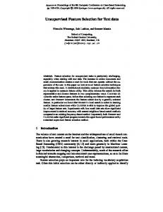
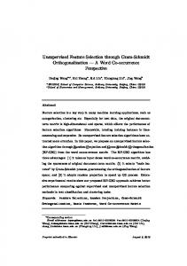
Yahoo! provides historical stock prices for the S&P 500 Index [44]. We collected historical prices for the 500 stocks of the index from Jan 2, 2003 to August 1, 2007, a total of 1153 days. Thus we constructed an 1153×500 date-by-stock matrix. The (i, j)-th element of this matrix represents the value of the j-th stock at the i-th day. We discarded 19 stocks that had missing values for a large number of dates, and we were left with a 1153 × 481 matrix. We normalized this matrix by computing z-scores for each column and we report results on this normalized date-by-stock matrix. The resulting matrix is quite low-rank from a numerical perspective. In particular, we experimented with three different choices for k = 10, 15, 20; notice that they correspond to approximately 2.5%, 3.5%, and 5% of the non-zero singular values of the matrix. However, the top 10, 15, and 20 singular values capture a significant percentage of the Frobenius norm of the matrix: 89%, 92%, and 94% respectively. In all three cases, the hybrid method consistently outperforms the corresponding deterministic method, and in many cases significantly so. See Figures 1 and 2 for a comparison between our hybrid approach and deterministic strategies for k = 10 and 20; k = 15 returned intermediate results and is not shown here. A few remarks are necessary. First, the gains of employing the hybrid approach are more pronounced for the smallest choice of k = 10. As k grows, the performance of our hybrid algorithm drops; for example, for k = 20, our algorithm does not outperform the Low RRQR algorithm. This seems to agree with our theoretical bound, which worsens as k grows. For example, notice that if k is a constant fraction of n, our theoretical result does not outperform the existing bounds for the CSSP. Second, the choice of the number of columns that are selected in the randomized step of our approach is important. Our theoretical result necessitates that O(k log k) columns of A are picked in the randomized step2 . On the other hand, the performance of the deterministic step drops if the number of columns picked in the randomized step increases. Thus, there exists an optimal choice for the parameter c in the randomized step. This optimal choice is – asymptotically – O(k log k). This manifests itself in the plots: at some point, picking more columns in the randomized step results to diminished performance. In most cases, setting c to be a small constant times k suffices for accurate approximations. Indeed, a practical implementation of our approach should “explore” a small number of choices for c, say c = 2k up to c = 10k in increments of k. Third, Low

1. Pivoted QR: We employed Matlab’s qr function. This function implements the algorithm described by Golub in [22]; the best known bound for the spectral norm of the residual error for this algorithm is proved in [24]: √ kA − PC Ak2 ≤ n − k2k kA − Ak k2 . 2. SPQR: The Semi Pivoted QR (SPQR) method described by Stewart in [38]. A Matlab implementation is available from [3]. We are not aware of provable a priori bounds for this algorithm. 3. High RRQR: High RRQR was devised by Chan in [8]. A MatLab implementation is available from [17]. The best known bound for the spectral norm of the residual error for this algorithm is: p kA − PC Ak2 ≤ k(n − k)2n−k kA − Ak k2 . 4. Low RRQR: Low RRQR was proposed by Chan and Hansen in [10]. A MatLab implementation is available from [17]. The best known bound for the spectral norm of the residual error for this algorithm is: p kA − PC Ak2 ≤ (k + 1)n2k+1 kA − Ak k2 . 5. qrxp: qrxp is the algorithm implemented as the LAPACK routine DGEQPX in ACM Algorithm 782 [5, 4]. We will use the MatLab implementation of the Fortran routine DGEQPX from [19]. The best known bound for the spectral norm of the residual error for this algorithm is: p kA − PC Ak2 ≤ 4 (k + 1)(n − k) kA − Ak k2 . 6. qryp: qryp is the algorithm implemented as the LAPACK routine DGEQPY in ACM Algorithm 782 [5, 4]. We will use the Matlab implementation of the Fortran routine DGEQPY from [19]. The best known bound for the spectral norm of the residual error for this algorithm is: p kA − PC Ak2 ≤ (10/9) (k + 1)2 (n − k) kA − Ak k2 . The platform used was a 2.0 GHz Pentium IV with 1GB RAM. Our code was implemented in MatLab 7.0.1. In this extended abstract we do not report running times for the different approaches, since they are less interesting than the accuracy results. However, all approaches run in comparable running times, with our approach being slower by small constant factors (three to five), mainly due to the 40 repetitions in Algorithm 1.

2 Pinning down the exact constant in the big-Oh notation seems quite hard given state of the art results for approximate matrix multiplication that are used in our proof.

65

0

0

50

100 150 200 250 300 350 400 number of columns kept in the randomized phase

450

qrxp 2−phase algorithm SVD

2

1

0

0

50

100 150 200 250 300 350 number of columns kept in the randomized phase

400

High RRQR 2−phase algorithm SVD

2

1

0

0

50


400

Low RRQR 2−phase algorithm SVD

2

1

0

0

50


400

spectral norm residual error


3

1



3

2

4

4



3

Pivoted QR 2−phase algorithm SVD

4



3

4

Pivoted QR 2−phase algorithm SVD

3 2 1 0 50

100


450

500

SPQR 2−phase algorithm SVD

3 2 1 0 50

100


450

500

qryp 2−phase algorithm SVD

3 2 1 0 50

100


450

500

Low RRQR 2−phase algorithm SVD

3 2 1 0 50

100


450

500

Figure 1: Comparison of our algorithm with four deterministic strategies and the SVD for k = 10. The y-axis is normalized so that the spectral error of the best rank-k approximation corresponds to one.

Figure 2: Comparison of our algorithm with four deterministic strategies and the SVD for k = 20. The y-axis is normalized so that the spectral error of the best rank-k approximation corresponds to one.

RRQR (despite the lack of strong theoretical guarantees) turns out to be a solid deterministic strategy for the column subset selection problem for small and medium values of k. In particular, our hybrid algorithm only marginally outperforms it for k = 10 and k = 15, and does not outperform it for k = 20. Our unsupervised column selection methodology picks k stocks that essentially have the same spectral norm residual as the top k left singular vectors. However, it is not easy to assign a meaning to the selected stocks, partly because a natural interpretation of the top k principal components in financial terms is not obvious. In particular, stocks in the S&P 500 index are separated in ten sectors, e.g., Industrial, Health Care, Consumer Discretionary, Financial, Information Technology, Utilities, Materials, Consumer Staples, Energy, and Telecommunication Services. However, when we examined the projection of the stock matrix on its top ten (or up to 20) singular vectors, we were not able to, for example, match the axes corresponding to singular vectors to sectors. Reifying the principal components of this data matrix seemed hard, hence assigning a meaning to the selected stocks is not straightforward. Table 3 shows the stocks that achieved the minimal residual error among all six methods and all different numbers of columns kept in the randomized step. This result was observed using the qrxp method with

c set to 160 for the randomized step. Notice that four stocks from the Industrials sector were picked; this seems to agree with the fact that this particular sector is quite diverse, and its behavior is representative of the S&P 500 as a whole.

4.3

TechTC datasets

Our second data application comes from the Open Directory Project (ODP) [32], a multilingual open content directory of WWW links that is constructed and maintained by a community of volunteer editors. ODP uses a hierarchical ontology scheme for organizing site listings. Listings on similar topics are grouped into categories, which can then include smaller subcategories. Gabrilovich and Markovitch constructed a benchmark set of term-document matrices from ODP, called TechTC (Technion Repository of Text Categorization Datasets [21]), which they made publicly available. Each matrix of the TechTC dataset consists of a total of 150 to 200 documents from two different ODP categories. The category that each document belongs to was also made available. As expected, the TechTC matrices are not numerically low-rank. The top 2.5%, 3.5%, and 5% of the non-zero singular values of these matrices capture (on average) 5.5%, 8%, and 12.5% of the Frobenius norm of the matrices. This is to be contrasted with the same values for the S&P 500 matrix, where 90% or more of the Frobenius

66

Stock Name TECO Energy Rowan Cos. Citrix Systems AFLAC Inc. Teradyne Inc. PACCAR Inc. Tyco C.H. Robinson Caterpillar Inc. Stanley Works

Sector Utilities Energy Inf. Tech. Financials Inf. Tech. Industrials Industrials Industrials Industrials Consumer Disc

0.2 id1 = 11346 id2 = 22294

0.15

0.1

0.05 Second singular vector

Stock symbol TE RDC CTXS AFL TER PCAR TYC CHRW CAT SWK

0

−0.05

−0.1

−0.15

Table 3: The ten stocks that minimized the spectral norm residual for k = 10.

−0.2

−0.25

(i) florida, evansville, their, consumer, reports (ii) diego, evansville, pianos, which, services (iii) florida, nanaimo, served, expensive, other (iv) eureka, california, cobbler, which, insurance (v) eureka, reliable, coldwell, rosewood, information (vi) dallas, nanaimo, untitled, buffet, included (vii) nanaimo, taiwan, megahome, great, states (viii) agent, topframe, spacer, order, during (ix) dublin, beach, estate, spacer, which (x) canada, stone, mainframe, spacer, other

−0.3

0

0.05

0.1

0.15

0.2 0.25 Top singular vector

0.3

0.35

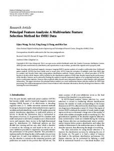
Figure 3: Projection of documents from the 1134622294 categories of the TechTC dataset onto the top two left singular vectors. in our study. Table 4 shows the terms that minimized the spectral norm residual using our hybrid algorithm. Obviously, the selected terms correlate reasonably well with the content of each dataset. In particular, in most cases we pick words that describe the content of each cluster of documents represented in the data.

Table 4: Retrieved terms norm of the matrix was captured with the same ratio of singular values. We note here that we preprocessed all matrices by removing all words with at most four letters. Despite this fact, we noticed that at least a few of the 100 matrices had the following property: the documents clustered well when projected in a low dimensional space spanned by the top few (e.g., four or five) left singular vectors. We empirically measured this property by computing low-rank approximations for all 100 matrices, and then applying k-means to the low-dimensional data. After measuring the quality of the resulting clustering when compared with the available ground truth, we focused on ten datasets where unsupervised clustering techniques performed well in predicting the two distinct clusters. This separation implies that the documents are semantically well-represented by low-rank approximation via the SVD, even though they are not numerically low-rank. Since our goal is to discuss unsupervised feature selection, we focused only on these matrices. Figure 3 shows a projection of one of the ten matrices on its top two left singular vectors. Notice that even in a 2D space some separation of the two classes is obvious. This separation typically peaks when four or five singular vectors are chosen. For simplicity and uniformity we always set the parameter k of our algorithm to five. The numerical results of our experiments are very similar to the ones for the S& P 500 and are omitted. Once more, we observe that our hybrid method outperforms most of the deterministic strategies3 . Table 5 shows some statistics for the ten document-term matrices that we included

4.4

HapMap dataset

It is well-known that genetic markers can be used to infer population structure and individual ancestry, two tasks that remain central challenges in many areas of genetics such as population genetics and the search of susceptibility genes for common disorders. The Singular Value Decomposition has recently regained favor for uncovering population structure, since it can be efficiently used to extract the fundamental structure of a dataset without the need for any modeling of the data; see [36] and references therein for a detailed discussion. SVD and PCA were first used in population genetics by Cavalli-Sforza to infer axes of human variation [30]. Selecting the appropriate genetic markers to study is critical. Single Nucleotide Polymorhisms (SNPs) are the most abundant forms of genetic variation. Each individual carries two identical or distinct copies (alleles) for a given SNP. Each copy is one of (at most) two alternate nucleotides that may appear at any given SNP. The HapMap Project [41] has genotyped millions of SNPs across the whole genome for certain populations. Identifying a minimal set of markers that could effectively be used for inference of population structure will reduce genotyping costs. Several approaches have been used to this end; see [35] for a detailed discussion. In all cases, knowledge of individual membership to a studied population is a prerequisite. When studying admixed populations it may be difficult to define or sample the ancestral populations. The origin of the study individuals may also be unknown in studies involving large samples of blood donors. In matrix language, our data consisted of n surveyed SNPs for m individuals. In the dataset that we will analyze here, n ≈ 2, 000, 000 and m = 90. Our 90 individuals come from a Chinese population and a Japanese population. The en-

3 We should note that the available implementations of the High and Low RRQR methods did not run in these datasets. The available code is designed for matrices with fewer columns than rows, and ran out of memory for the TechTC matrices.

67

0.4

1

id2 11346 2 12121 3 22294 4 14517 6 186330 7 22294 4 25575 9 61792 11 814096 12 90753 14

Separating CHB and JPT using the top singular vector

#docs × #terms 139 × 15170 138 × 11859 125 × 14392 125 × 15485 130 × 18289 130 × 12708 127 × 10012 159 × 15860 159 × 16066 154 × 14780

0.15

0.1

0.05

Top singular vector

(i) (ii) (iii) (iv) (v) (vi) (vii) (viii) (ix) (x)

id1 10567 1 10567 1 11346 2 11498 5 14517 6 20186 8 22294 4 332386 10 61792 11 85489 13

0

−0.05

−0.1

−0.15

US: Indiana: Evansville US: Florida 3 California: San Diego: Business, economy 4 Canada: British Columbia: Nanaimo 5 California: Politics: Candidates, campaigns 6 US: Arkansas 7 US: Illinois 8 US: Texas: Dallas 9 Asia: Taiwan: Business and Economy 10 Shopping: Vehicles 11 US: California 12 Europe: Ireland: Dublin 13 Canada: Business and Economy: Industries 14 Materials and Supplies: Masonry and Stone 2

Chinese Japanese −0.2

0

10

20

30

40 50 Individuals

60

70

80

90

Figure 4: Individuals of Chinese and Japanese ancestry from HapMap projected on the top singular vector. Keeping 40 SNPs Number of misclassifications

50

Table 5: The 10 TechTC matrices of our study.

Uniform sampling (10 reps) Hybrid approach (10 reps) Informativeness

40 30 20 10 0

500

1000 1500 2000 Number of SNPs selected in randomized phase

2500

Keeping 50 SNPs Number of misclassifications

50

tries in the m × n matrix are +1 (if both alleles are equal to the first nucleotide), −1 (if both alleles are equal to the second nucleotide), or 0 (if the two alleles are different). The task at hand is to identify a small set of SNPs (columns) and/or individuals (rows) that capture the structure of the data, e.g., that suffice to accurately assign an individual to a population of origin. We will seek to do this in an unsupervised manner, e.g., by selecting the most representative SNPs without any a priori knowledge of individual ancestry. Once more, the given matrix is not numerically low-rank. In particular, the top 2.5%, 3.5%, and 5% of the non-zero singular values of our matrix capture 3%, 7%, and 13% of its Frobenius norm. Figure 4 shows a projection of our data (after mean-centering) in the top left singular vector of the matrix A. Clearly, the Chinese and Japanese individuals are well separated, with the exception of a single Japanese subject who lies in the middle. Our goal is to find a small subset of SNPs that reproduce this structure using our hybrid approach. In order to reduce the running time to a few minutes, we modified Algorithm 1 to perform only ten repetitions. Given the huge number of columns, none of the existing codes for deterministic methods could run without heavy modifications. Since in this case k is equal to one, we are essentially seeking a single column that minimizes the residual error when the whole matrix A is projected on the chosen column. This objective is clearly mundane: first, since k is equal to one, we could solve the whole problem exhaustively (albeit in O(mn2 ) time with n ≈ 2, 000, 000). Most importantly, the goal of a geneticist is to identify a small set of SNPs (not necessarily one) that suffices to determine the ancestry of an individual. Hence, a much more meaningful evaluation

Uniform sampling (10 reps) Hybrid approach (10 reps) Informativeness

40 30 20 10 0

500

Figure 5: SNPs.

1000 1500 2000 2500 Number of SNPs selected in randomized phase

3000

Classification accuracy using selected

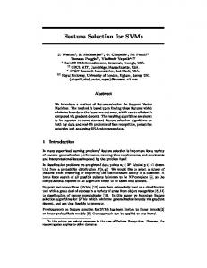
of our feature selection algorithm is to examine the performance of the selected SNPs in separating individuals of Chinese and Japanese ancestry. Figure 5 shows the performance of k-means applied on a very small (e.g., 40 or 50 out of 2,000,000) set of SNPs selected using our hybrid algorithm. Notice that selecting 40 SNPs and using them to cluster the 90 individuals in two clusters results to about 7 misclassifications when 1,000 SNPs are selected in the randomized phase. Similarly, 50 SNPs result to only 4 misclassifications when 1,500 SNPs are selected in the randomized phase. When compared to the best existing supervised method for the same task (the measure of Informativeness for assignment defined by Rosenberg in [37]), as well as randomly chosen SNPs, we can easily see that our unsupervised algorithm is essentially as good as the best existing supervised method.

5.

FUTURE DIRECTIONS

It would be particularly interesting to design unsupervised feature selection algorithms for other, non-linear, dimensionality reduction methods. In recent years, we witnessed

68

an explosion in the design of non-linear dimensionality reduction algorithms, including Laplacian Eigenmaps, Locally Linear Embedding (LLE), IsoMap, SemiDefinite Embedding (SDE), diffusion geometries, etc. In words, dimensionality reduction techniques seek to compress the data while keeping all the relevant structure intact. An important open problem is the development of efficient, unsupervised, and provably accurate approaches that select a subset of features from the data such that running the dimensionality reduction algorithm only on this subset of features, as opposed to the full set of features, achieves essentially the same reconstruction.

6.

[21] E. Gabrilovich and S. Markovitch. Text categorization with many redundant features: using aggressive feature selection to make SVMs competitive with C4.5. ICML, 2004 [22] G. H. Golub. Numerical methods for solving linear least squares problems. Numer Math, 7:206–216, 1965. [23] G.H. Golub and C.F. Van Loan. Matrix Computations. Johns Hopkins University Press, Baltimore, 1989. [24] M. Gu and S.C. Eisenstat. Efficient algorithms for computing a strong rank-revealing QR factorization. SIAM J Sci Comp, 17:848–869, 1996. [25] Y. P. Hong and C. T. Pan. Rank-revealing QR factorizations and the singular value decomposition. Math Comp, 58:213–232, 1992. [26] W. J. Krzanowski. Selection of variables to preserve multivariate data structure, using principal components. Applied Statistics, 36(1):22–33, 1987. [27] F.G. Kuruvilla and P.J. Park and S.L. Schreiber. Vector algebra in the analysis of genome-wide expression data. Genome Biology, 3, 2002. [28] K. Z. Mao. Identifying critical variables of principal components for unsupervised feature selection. IEEE Transactions on Systems, Man, and Cybernetics, Part B, 35(2):339–344, 2005. [29] M.W. Mahoney, M. Maggioni, and P. Drineas. Tensor-CUR decompositions for tensor-based data, KDD, 2006. [30] P. Menozzi, A. Piazza, and L. Cavalli-Sforza. Synthetic maps of human gene frequencies in Europeans . Science, 201(4358):786–792, 1978. [31] P. Mitra, C. A. Murthy, and S. K. Pal. Unsupervised feature selection using feature similarity. IEEE Trans. Pattern Anal. Mach. Intell., 24(3):301–312, 2002. [32] Open Directory Project. http://www.dmoz.org/ [33] C. T. Pan. On the existence and computation of rank-revealing LU factorizations. Linear Algebra Appl, 316:199–222, 2000. [34] C. T. Pan and P. T. P. Tang. Bounds on singular values revealed by QR factorizations. BIT Numerical Mathematics, 39:740–756, 1999. [35] P. Paschou, E. Ziv, E.G. Burchard, S. Choudhry, W.R. Cintron, M.W Mahoney, and P. Drineas. PCA-Correlated SNPs for Structure Identification in Worldwide Human Populations, PLoS Genetics, 9(3), 2007. [36] P. Paschou, M.W. Mahoney, A. Javed, J.R. Kidd, A.J. Pakstis, S. Gu, K.K. Kidd, and P. Drineas. Intra- and Inter-population genotype reconstruction from tagging SNPs, Genome Research, 17: 96-107, 2007. [37] N.A. Rosenberg, L.M. Li, R. Ward, and J.K. Pritchard. Informativeness of genetic markers for inference of ancestry. Am J Hum Genet, 73(6):1402–1422, 2003. [38] G.W. Stewart. Four algorithms for the efficient computation of truncated QR approximations to a sparse matrix. Num Math, 83:313–323, 1999. [39] H. Stoppiglia, G. Dreyfus, R. Dubois, and Y. Oussar. Ranking a random feature for variable and feature selection. J. Mach. Learn. Res., 3:1399–1414, 2003. [40] J. Sun, Y. Xie, H. Zhang, and C. Faloutsos. Less is more: Compact matrix decomposition for large sparse graphs, SDM, 2007. [41] The International HapMap Consortium. A haplotype map of the human genome. Nature, 437:1299–1320, 2005. [42] L. Wolf and A. Shashua. Feature selection for unsupervised and supervised inference: The emergence of sparsity in a weight-based approach. J. Mach. Learn. Res., 6:1855–1887, 2005. [43] Z. Zhao and H. Liu. Spectral feature selection for supervised and unsupervised learning. In ICML, 2007. [44] http://finance.yahoo.com/

REFERENCES

[1] A. d’Aspremont, L. El Ghaoui, M. I. Jordan, and G. R. G. Lanckriet. A Direct Formulation for Sparse PCA Using Semidefinite Programming. SIAM Review, 49(3), July 2007 [2] A. Ben-Hur and I. Guyon. Detecting stable clusters using principal component analysis. Methods Mol Biol, 224:159–182, 2003. [3] M.W. Berry, S.A. Pulatova, and G.W. Stewart. Computing sparse reduced-rank approximations to sparse matrices. ACM Trans on Math Soft, 31:252–269, 2005. [4] C. H. Bischof and G. Qintana-Ort´ı. Algorithm 782: codes for rank-revealing QR factorizations of dense matrices. ACM Trans on Math Soft, 24:254–257, 1998. [5] C.H. Bischof and G. Quintana-Ort´ı. Computing rank-revealing QR factorizations of dense matrices. ACM Trans on Math Soft, 24(2):226–253, 1998. [6] C. Boutsidis, M.W. Mahoney, and P. Drineas. Manuscript in preparation, 2008 [7] J. Cadima, J. O. Cerdeira, and M. Minhoto. Computational aspects of algorithms for variable selection in the context of principal components. Computational Statistics & Data Analysis, 47(2):225–236, 2004. [8] T. F. Chan. Rank revealing QR factorizations. Linear Algebra Appl, 88/89:67–82, 1987. [9] T.F. Chan and P.C. Hansen. Some applications of the rank revealing QR factorization. SIAM J Sci and Stat Comp, 13:727–741, 1992. [10] T. F. Chan and P.C. Hansen. Low-rank revealing QR factorizations. Linear Algebra Appl, 1:33–44, 1994. [11] S. Chandrasekaran and I. C. F. Ipsen. On rank-revealing factorizations. SIAM J Matrix Anal Appl, 15:592–622, 1994. [12] A. Deshpande, L. Rademacher, S. Vempala, and G. Wang. Matrix approximation and projective clustering via volume sampling. SODA, 2006 [13] M. Devaney and A. Ram. Efficient feature selection in conceptual clustering. In ICML, 1997. [14] P. Drineas, M. W. Mahoney, and S. Muthukrishnan. Subspace sampling and relative-error matrix approximation: Column-based methods, APPROX-RANDOM, 2006. [15] P. Drineas, M. W. Mahoney, and S. Muthukrishnan. Relative-error CUR matrix decompositions. http://arxiv.org/abs/0708.3696, 2007. [16] J G. Dy and C E. Brodley. Feature selection for unsupervised learning. J. Mach. Learn. Res., 5:845–889, 2004. [17] R.D. Fierro, P.C. Hansen, and P. Hansen. UTV tools: Matlab templates for rank-revealing UTV decompositions. Numerical Algorithms, 20(2-3):165–194, 1999. [18] L. V. Foster. Rank and null space calculations using matrix decomposition without column interchanges. Linear Algebra Appl, 74:47–71, 1986. [19] L.V. Foster and Xinrong Liu. Comparison of rank revealing algorithms applied to matrices with well defined numerical ranks. manuscript, 2006. [20] A. Frieze, R. Kannan, and S. Vempala. Fast Monte-Carlo algorithms for finding low-rank approximations, FOCS, 1998

69