Session 1. Statistic Methods and Their Applications
Proceedings of the 12th International Conference “Reliability and Statistics in Transportation and Communication” (RelStat’12), 17–20 October 2012, Riga, Latvia, p. 20–26. ISBN 978-9984-818-49-8 Transport and Telecommunication Institute, Lomonosova 1, LV-1019, Riga, Latvia
USE OF STATISTICAL TECHNIQUES FOR CRITICAL GAPS ESTIMATION Andrea Gavulová University of Žilina, Faculty of Civil Engineering Department of Highway Engineering Univerzitná 8251/1, SK-010 26 Žilina, Slovak Republic Ph.:+421 41-513 9512. E-mail:
[email protected] The critical gap is very important parameter for capacity calculation of unsignalized intersections. This parameter is a stochastically distributed value and it cannot be measured directly on the field. Only rejected gaps and accepted gaps of each minor stream vehicle can be measured at the intersection. Consequently, some statistical model or procedure for estimating critical gaps is needed. There are many different methods or procedures for critical gap estimation and many studies about estimating the critical gap have been carried out. But in Slovakia we have only a little practical experiences because similar studies have rarely been done in our country. This paper presents a short overview of three methods for the estimation of critical gaps at unsignalized intersections: method of Raff (1950), Maximum Likelihood Method (MLM) of Troutbeck (1992) and method of Wu (2006). These methods are presented on a practical example. Input date – observed accepted and maximum rejected gaps of each minor stream vehicle – were determined on the basis of video survey at the unsignalized intersection in Žilina. Critical gaps are estimated by using these three methods and results are compared each other. Keywords: critical gap estimation, rejected and accepted gap, maximum likelihood method, probability, unsignalized intersection
1. Introduction Methods of capacity calculation for unsignalized intersections are mostly based on Gap acceptance procedure (GAP). In this procedure the critical gap is an important parameter for capacity calculation. There are different values of critical gaps for drivers in different geometry and traffic conditions. The problem is the critical gaps cannot be measured directly. Only reject gaps and accepted gaps of single vehicles in the minor stream can be measured at the intersection. Consequently, some statistical model or procedure for estimating critical gaps at unsignalized intersections is needed. There are many different methods or procedures for critical gap estimation (more than 20 methods), such as method of Raff (1950), Harders (1968), Aworth (1970), Siegloch (1973), Troutbeck (1992) and so on. The most commonly used methods for estimating the critical gap are the method of Raff (1950) and Troutbeck (1992). The method of Raff (1950) is based on macroscopic model and it is the earliest method for estimating the critical gap which is used in many countries because of its simplicity. In Troutbeck's microscopic model the probability of the critical gap is calculated through the Maximum Likelihood Method (MLM).An iteration process is necessary. The outcome of Brilon et al. comprehensive analyses [1] is MLM of Troutbeck (1992) gives the best results. This method is recommended for estimating the critical gaps in the best-known standard manuals for traffic engineering HCM 2000 and HBS 2001. Unfortunately, the model of Troutbeck (1992) is very complicated to common use for traffic engineers. Besides the mentioned methods, Wu (2006) developed a macroscopic method based on equilibrium of probabilities between the rejected and accepted gaps [2]. Using this method is simple; it can be carried out easy by spreadsheet programs without iterations. This paper briefly introduced method of Raff (1950), MLM of Troutbeck (1992) and method of Wu (2006). In Slovakia we have only a little practical experiences about estimating the critical gap because similar studies have rarely been done in our country. This paper presents practical example of critical gaps estimation by using these three methods. The critical gaps were calculated and compared each other. Input date (accepted gaps and maximum rejected gaps) were determined on the basis of video survey at the unsignalized intersection in Žilina.
20
The 12th International Conference “RELIABILITY and STATISTICS in TRANSPORTATION and COMMUNICATION - 2012”
2. Methods for Estimating the Critical Gap The critical gap tc can be defined as the minimum time interval between the major stream vehicles that is necessary for one minor stream vehicle to make a maneuver (see Figure 1).Values of critical gaps are different for different drivers (some of them are too fast or risky, some of them are slow or careful) and there are dependent on types of movements, geometry parameters of intersections, traffic situation. Due to this variability gap acceptance process is consider as a stochastic process and the critical gaps are random variables. The estimation of critical gaps tries to find out values for the variables and as well as for the parameters of their distributions, which represent typical driver behavior at the investigated intersection.
Figure 1. The critical gap for minor stream right-turn vehicle
In unsignalized intersection theory it is generally assumed that drivers are both consistent and homogeneous. Consistent drivers are expected to behave the same way every time in all similar situations. This means: a driver with a specific tc-value will never accept a gap less than tc and he will accept each major stream gap larger than tc. However, within a population of several drivers, each of which behaves consistent, different drivers could have their own tc-value. These tc-values are then treated as a random variable with a special statistical density function ftc(t)and cumulative distribution function Ftc(t). The population of drivers is homogeneous if each sub-group of drivers out of the population has the same functions ftc(t)and Ftc(t). The problem is that the critical gaps cannot be measured directly. Only rejected gaps and accepted gaps of each minor stream vehicle can be measured at the intersection. The critical gaps can be estimated from these input data using some statistical method or procedures. For the estimation of critical gaps from observations three methods are briefly described in this article and applied in a practical example – method of Raff (1950), Maximum Likelihood Method (MLM) of Troutbeck (1992) and method of Wu (2006). 2.1. The Raff´s Method The method of Raff (1950) is based on macroscopic model and it is the earliest method for estimating the critical gap which is used in many countries because of its simplicity. This method involves the empirical distribution functions of accepted gaps Fa(t) and rejected gaps Fr(t). When the sum of cumulative probabilities of accepted gaps and rejected gaps is equal to 1 then a gap of length tis equal to critical gap tc. It means the number of rejected gaps larger than critical gap is equal to the number of accepted gaps smaller than critical gap. (1)
Fa (t ) = 1 − Fr (t ) . 2.2. The Maximum Likelihood Method
The model of Troutbeck (1992) for estimating critical gaps is based on the Maximum Likelihood Method (MLM). This microscopic model assumes the log-normal distribution of accepted and maximum rejected gaps. In this model, only the accepted gap and the maximum rejected gap of each vehicle are
21
Session 1. Statistic Methods and Their Applications
treated pair wise. For one individual minor street driver i we have observed: one accepted gap ai and one corresponding the maximum rejected gap ri. The maximum rejected gap is the largest value of all rejected gaps for one minor street driver. The MLM is based on the assumption that minor stream drivers behave consistently. It means that each driver will reject every gap smaller than his critical gap and will accept the first gap larger than the critical gap. Under this assumption, the distribution of the critical gaps lies between distributions of largest rejected and accepted gaps (see Figure 2). The parameters of distribution function of the critical gaps, the mean µ and variance σ2, are obtained by maximizing the likelihood function. The likelihood function is defined as the probability that the critical gap distribution lies between the observed distribution of the maximum rejected gaps and the accepted gaps: n
∏ [F (a ) − F (r )] , i
(2)
i
i =1
where L ai ri F(ai), F(ri)
– maximum likelihood function, – logarithm of the accepted gap of driver i, – logarithm of the maximum rejected gap of driver i, – cumulative distribution functions for the normal distribution.
Figure 2. Theoretical distribution function of accepted gaps Fa(t), maximum rejected gaps Fr(t), and critical gaps Ftc(t)
The logarithm of function (3) is as follows: n
L = ∑ ln[F ( ai ) − F (ri )] .
(3)
i =1
Likelihood parameters µ and σ2 are solutions when the partial derivative of equation (4) is equal to 0. They can be simplified as follows:
n f ( ai ) − f (ri ) − ∑ F ( a ) − F ( r ) = 0 i i i =1 , 1 n (a − µ ). f ( a ) − ( r − µ ). f (r ) i i i i − =0 2 ∑ F (ai ) − F (ri ) 2σ i =1
(4)
where f(ai), f(ri) – probability density functions for the normal distribution with parameters µ and σ2. Parameters µ and σ2 can be calculated by numerical and iteration techniques [5]. Subsequently the mean E(tc) and variance D(tc) of critical gap can be derived by equations:
22
The 12th International Conference “RELIABILITY and STATISTICS in TRANSPORTATION and COMMUNICATION - 2012”
2
E (t c ) = e µ +0 ,5σ .
(5) 2
D(t c ) = E (t c ) 2 .(eσ − 1) .
(6)
2.3. The Model Based on the Macroscopic Probability Equilibrium The theoretical background of Wu´s model [2] is the probability equilibrium between the rejected and the accepted gaps. The equilibrium is established macroscopically from the cumulative distribution of the rejected and accepted gaps. The observed probability that a gap of length t is accepted is Fa(t) and that it is not-accepted is 1–Fa(t). The observed probability that a gap of length t is rejected is Fr(t) and that it is not-rejected is 1–Fr(t). Generally Fr(t) ≠ 1–Fa(t) and 1–Fr(t) ≠ Fa(t). Considering the observed probability of both – acceptance and rejection, Wu’s method is based on the following probability equilibrium: (7)
Pr ,tc (t ) = Fr (t ) ⋅ Pr ,tc (t ) + Fa (t ) ⋅ Pa ,tc (t ) .
Denote the distribution function of the critical gaps to be estimated by Ftc(t), then the probability Pr,tc(t) that a gap of length t in the major stream would be rejected is Ftc(t), and the probability that it would be accepted is 1–Ftc(t). Substituting Pr,tc(t)=Ftc(t) and Pa,tc(t)=1–Ftc(t), for Wu´s model we have the following distribution function Ftc(t) of the critical gaps:
Ftc (t ) =
Fa (t ) 1 − Fr (t ) . = 1− Fa (t ) + 1 − Fr (t ) Fa (t ) + 1 − Fr (t )
(8)
For implementing the proposed macroscopic model of Wu is detailed calculation procedure step by step given in [2]. This procedure is easily implemented into Excel spreadsheet. According to Raff´s definition for the critical gap (Equation (1)) it can be written [2]:
Ftc (t ) =
Fa (t ) 1 − Fr (t ) . = 1− Fa (t ) + 1 − Fr (t ) Fa (t ) + 1 − Fr (t )
(9)
It means that the critical gap estimated from Raff´s method is the median value but not the mean value of the critical gap.
3. Practical Example of Estimating the Critical Gaps 3.1. Results of Measurements Measurements were carried out at the unsignalized intersections in Žilina. All traffic streams at this intersection were video-recorded. Subsequently video-recordings were processed by own specific software (using MATLAB).Time position of each vehicle on a certain point (designed line across the road) was recorded in a spread sheet MS Excel with accuracy 0,04 s (frame rate of camera: 25 frames per sec.). For each minor stream vehicle was recorded: arrival time, vehicle type, direction and departure time. For each major stream vehicle was recorded: passing time a designed line across the road, vehicle type and direction. All data were processed. The accepted and largest rejected gaps for individual minor stream vehicle were determined (for each minor stream separately). If a driver from minor stream accepted the lag and did not reject any time gap: a largest rejected time gap was equal 0 s. Example of estimating critical gaps of a minor left-turn stream at unsignalized intersection in Žilina (see Figure 3) by three estimating methods using statistical techniques (Raff, MLM and Wu) is given in this article. Traffic survey was carried out by video recording in durance one hour (peak hour).All observed input data – accepted and the maximum rejected gaps for each minor stream left-turn vehicle are presented on Figure 4. Two simples for estimating critical gaps have been given. In simple 1 there are not considered vehicles which had the maximum rejected gap equal to zero, so 80 couples of accepted and maximum rejected gaps were derived for estimating critical gap by all three methods. In simple 2 there are also considered vehicles which immediately entered to intersection without waiting and for estimating critical gap were derived 80 rejected gaps and 103 relevant accepted gaps. Data from simple 2 were used only for two macroscopic methods of Raff and Wu, because of requirement of MLM to have couples of accepted and maximum rejected gaps for estimation of critical gaps.
23
Session 1. Statistic Methods and Their Applications
Figure 3. Monitored unsignalised intersection in Žilina
Figure 4. Measurements of the maximum rejected gaps and accepted gaps (Data: Žilina 2012, minor stream left-turn)
3.2. Estimation and Comparison of Critical Gaps Results of Raff´s method The curves of accumulative probability of accepted gaps Fa(t) and maximum rejected gaps Fr(t) are shown on Figure 5. The critical gap tc = 5,80 s is in cross point of Fa(t)and 1–Fr(t). The critical gap was estimated by Raff´s model also considering all accepted gaps from input data (simple 2). Although distribution function Fa(t) for simple 2 is slightly different to Fa(t) for simple 1, cross point is in the same gap time, the critical gap tc = 5,80 s. Results of MLM of Troutbeck In accordance with MLM of Troutbeck the probability density functions of accepted gaps f(ai) and maximum rejected gaps f(ri), distribution functions of accepted gaps F(ai) and maximum rejected gaps F(ri) were calculated for each logarithm of accepted gap ai and logarithm of maximum rejected gap ri. The likelihood parameters: the mean µ and variance σ2, were obtained as a solution of two equations (4) by iteration process. The iteration process was programmed in Excel program. Values µ and σ2 where changed step by step until functions in equation (4) tend to zero. Finally the mean E(tc) = 6,04 s and variance D(tc) = 5,38 s2 of critical gap were derived by equations (5) and (6).
Figure 5. The critical gap estimation by Raff´s method, distribution functions of the maximum rejected gaps – Fr(t) and accepted gaps – Fa(t) for simple 1 and simple 2
24
The 12th International Conference “RELIABILITY and STATISTICS in TRANSPORTATION and COMMUNICATION - 2012”
Results of macroscopic method of Wu The distribution functions of accepted gaps Fa(t) and maximum rejected gaps Fr(t) are shown on Figure 6. The distribution function of critical gap Ftc(t) was calculated in accordance with macroscopic probability equilibrium model of Wu by equation (8) and the curve of this function lies between Fa(t) and Fr(t). The mean value of the critical gap tc = 5,91 s and the variance σ2 = 2,89 s2 were calculated. The median value of the critical gap was also calculated and its value is equal to Raff critical gap (5,8 s). For comparison, distribution function of the estimated critical gap from MLM of Troutbeck – Ftc(t) [MLM] – is also shown on Figure 6. The critical gap was estimated by macroscopic model of Wu also considering all accepted gaps from input data (simple 2). The mean value of the critical gap tc = 5,60 s and the variance σ2 = 3,34 s2 were calculated.
Figure 6. Distribution functions of the maximum rejected gaps – Fr(t), accepted gaps – Fa(t), critical gaps from the Wu´s model – Ftc(t) [Wu] and distribution function of the estimated critical gap from MLM of Troutbeck – Ftc(t) [MLM]
4. Conclusions Maximum likelihood method of Troutbeck (1992) belongs to the most important models for estimating the critical gaps and according to [1] gives the best results. The macroscopic method of Wu (2006) gives similar results for the mean critical gaps as that from recognized MLM of Troutbeck (1992). In addition, we can get not only the main value of critical gaps but also the median value, which is the same value as the result of Raff´s method. Also we can directly get the probability distribution function of the critical gaps. Advantage of this method is simple calculation procedure without iteration as it is in the case of the Troutbeck model (1992). It can be carried out using spreadsheet programs, e.g. Excel, and therefore it is very useful for professionals of traffic engineering. In addition, not only couples of accepted and rejected gaps are required for estimation of critical gaps as in MLM of Troutbeck is required. It can be used all relevant accepted and maximum rejected gaps. In these cases the mean critical gap is shorter.
References 1. Brilon, W., König, R., Troutbeck, R. (1997). Useful Estimation Procedures for Critical Gaps. In Proceedings of the 3rd International Symposium on Intersections without Traffic Signals, July 21-23, 1997 (pp. 71-87). Portland Oregon, U.S.A: University of Idaho, National Center for Advanced Transportation Technology. 2. Wu, N. (2006). A new model for estimating critical gap and its distribution at unsignalized intersections based on the equilibrium of probabilities. In Proceedings of the 5th International Symposium on Highway Capacity and Quality of Services. July 25-29, 2006. Yokohama, Japan: Japan Society of Traffic Engineers. 3. Weinert, A. (2000). Estimation of Critical Gaps and Follow-Up Times at Rural Unsignalized Intersections in Germany. In Proceedings of the 4th International Symposium on Highway Capacity. June 27–July 1, 2000 (pp. 409-421). Maui, Hawaii: Transport Research Board.
25
Session 1. Statistic Methods and Their Applications
4. Guo, R. (2010). Estimating Critical Gap of Roundabouts by Different Methods. In Proceedings of the
6th Advanced Forum on Transportation of China 2010. October 16, 2010 (pp. 84-89). Beijing, China: Curran Associates, Inc. 5. Tian, Z., Vandehey, M., Robinson, B., Kittelson, W., Kyte, M., Troutbeck, R., Brilon, W., Wu, N. (1999). Implementing the maximum likelihood methodology to measure a driver´s critical gap. Transportation Research, Part A, 33, 187-197.
Acknowledgements This contribution is a result of the project‘s implementation: Centre of Excellence for Systems and Services of Intelligent Transport II, ITMS 26220120050 supported by the Research&Development Operational Programme funded by the ERDF.
"Podporujeme výskumné aktivity na Slovensku/Projekt je spolufinancovaný zozdrojov EÚ" ("We support research activities in Slovakia / The Project is co-funded by the EU")
26