United States Department of Agriculture Forest Service Rocky Mountain Research Station General Technical Report RMRS-GTR-96 September 2002
Users Guide to the Most Similar Neighbor Imputation Program Version 2 Nicholas L. Crookston Melinda Moeur David Renner
Partially inventoried planning area
Data Available for Some Sample Units
Data Available for All Sample Units Aerial Photo – Soils Map – Landsat TM – Digital Elevation Model –
Global Data
}
MSN
{
Planning area fully populated with inventory information using global data and estimates of ground data based on "most similar neighbors."
Ground-based Data
–Stand Exam –Fuels Inventory –Wildlife Habitat Survey
Abstract ______________________________________________ Crookston, Nicholas L.; Moeur, Melinda; Renner, David. 2002. Users guide to the Most Similar Neighbor Imputation Program Version 2. Gen. Tech. Rep. RMRS-GTR-96. Ogden, UT: U.S. Department of Agriculture, Forest Service, Rocky Mountain Research Station. 35 p. The Most Similar Neighbor (MSN, Moeur and Stage 1995) program is used to impute attributes measured on some sample units to sample units where they are not measured. In forestry applications, forest stands or vegetation polygons are examples of sample units. Attributes from detailed vegetation inventories are imputed to sample units where that information is not measured. MSN performs a canonical correlation analysis between information measured on all units and the detailed inventory data to guide the selection of measurements to impute. This report presents an introductory discussion of Most Similar Neighbor imputation and shows how to run the program. An example taken from a forest inventory application is presented with notes on other applications and experiences using MSN. Technical details of the way MSN works are included. Information on how to get and install the program and on computer system requirements is appended. The MSN Web address is: http://forest.moscowfsl.wsu.edu/gems/msn.html.
Keywords: canonical correlation, imputation, forest inventory, forest planning, landscape analysis
The Authors ___________________________________________ Nicholas L. Crookston is an Operations Research Analyst at the Moscow Forestry Sciences Laboratory. His contributions have included developing extensions to the Forest Vegetation Simulator. Melinda Moeur is the Vegetation Module Leader at the Interagency Monitoring Program, Northwest Forest Plan, Strategic Planning, Pacific Northwest Region, USDA Forest Service, Portland, OR. While she worked on this project she was a Research Forester at the Rocky Mountain Research Station’s Forestry Sciences Laboratory in Moscow, ID. Her principal research interests include forest vegetation modeling and sampling inference. David Renner is a freelance Computer Programmer in Moscow, ID. He has contributed to several projects at the USDA Forest Service, Rocky Mountain Research Station’s Moscow Laboratory related to FVS and its application. He also works at the University of Idaho and as a private forestry consultant.
You may order additional copies of this publication by sending your mailing information in label form through one of the following media. Please specify the publication title and number. Telephone
(970) 498-1392
FAX
(970) 498-1396
E-mail Web site Mailing Address
[email protected] http://www.fs.fed.us/rm Publications Distribution Rocky Mountain Research Station 240 West Prospect Road Fort Collins, CO 80526
Contents Page Introduction to Most Similar Neighbor Imputation ........................................................................... 1 Purpose ..................................................................................................................................... 1 Important Terms ........................................................................................................................ 2 Elements in an MSN Run .......................................................................................................... 2 A Simplistic Example ................................................................................................................. 3 New in Version 2 ........................................................................................................................ 4 What Follows ............................................................................................................................. 4 How to Run the Program ................................................................................................................. 4 Commands ................................................................................................................................ 4 Input Data Formats and Identifying Y- and X-Variables ............................................................ 7 Example Run Input .................................................................................................................. 10 Output ........................................................................................................................................... 13 Report File ............................................................................................................................... 13 For-Use File ............................................................................................................................. 23 Observed-Imputed File ............................................................................................................ 23 Factors that Influence MSN Imputations ....................................................................................... 24 Sampling .................................................................................................................................. 24 Choice of Variables .................................................................................................................. 25 Choice of Transformations ....................................................................................................... 26 Applications ................................................................................................................................... 26 Technical Details ........................................................................................................................... 28 Computing the Canonical Correlations .................................................................................... 28 Most Similar Neighbor Selection .............................................................................................. 28 Validation Statistics .................................................................................................................. 30 Acknowledgments ......................................................................................................................... 32 References .................................................................................................................................... 32 Appendix A: Program Installation and Computer Requirements ................................................... 34 Appendix B: Run Time Information ............................................................................................... 35
Users Guide to the Most Similar Neighbor Imputation Program Version 2 Nicholas L. Crookston Melinda Moeur David Renner
Introduction to Most Similar Neighbor Imputation _______________________ Purpose The Most Similar Neighbor (MSN, Moeur and Stage 1995) program is used to impute attributes measured on some sample units to sample units where they are not measured. A list of all sample units in a problem is constructed, and some attributes are measured for every unit. Additional attributes, typically those that are much more expensive to measure, are recorded for some of the units. The MSN program picks the most similar unit where the additional attributes are measured to impute to a unit where the additional attributes are not measured. Information about the relationship between the attributes measured for all units and the additional attributes measured on a sample of the units is compiled by the program using canonical correlation analysis and used to compute the similarity among units. An application in forestry serves to illustrate the idea. A list of all the forest stands in a large watershed is made. In this case each forest stand is a sample unit. Then, easy-to-measure attributes are recorded for all the forest stands in the watershed. These attributes can come from any source; aerial photographs and topographic maps are good examples. For a sample of the stands, attributes are measured during on-the-ground visits. The program picks the most similar stand that was visited on the ground to characterize a stand that was not visited. The technique was developed to support detailed, landscape-level analyses, required in today’s forest planning environment. Geographic Information systems (GIS) linked with databases that store inventory information about landscape elements provide the data tools needed to create these plans. Despite the availability of sophisticated display and database tools, a comprehensive landscape wide plan is still difficult to create because the inventory is rarely complete. In other words, even though a GIS can easily display all the planning units (such as forest stands) in an analysis area, rarely do all planning units have a ground-based inventory. For planning purposes, it would be convenient to be able to operate as if detailed inventory information were available for all units in the planning area. For units in a landscape that lack ground-based attributes, MSN can be used to find the most similar ground-based unit and impute its inventory attributes to the unit that lacks those data (Moeur and others 1995, Ek and others 1997, Van Deusen 1997).
USDA Forest Service Gen. Tech. Rep. RMRS-GTR-96. 2002
1
Crookston, Moeur, and Renner
Users Guide to the Most Similar Neighbor Imputation Program Version 2
Important Terms In the MSN system, all the units in a problem have some measured information and are therefore called observations. In MSN, as in databases or spreadsheets, an observation is a row in a table. The columns of the table are known as variables. In a forestry application, the observations might be stands, and an example variable is the number of trees per acre. A value is a cell in the table. Variables measured for all the observations in the MSN analysis are known as X-variables. The additional variables measured only for a sample of the observations are known as Y-variables. Common X-variables in forestry include those obtained from aerial photo interpretation such as crown closure, average tree height, species group, and stocking class. Variables derived from remotely sensed satellite spectral data and digital elevation models are also used. Common Y-variables include those obtained from stand examinations or similar vegetation inventories such as Forest Inventory and Analysis grid plots. Examples include the basal area, percent canopy cover, trees per acre, volume, species composition, and size class. Observations that have measured Y-variables and X-variables are called reference observations. Observations that lack measured Y-variables are called target observations. The objective of MSN is to pick a reference observation as a source of Y-variables to impute to a target observation. This is done by computing the weighted distances between each target observation and every reference observation. The reference observation with the shortest weighted distance between itself and a given target observation is the target observation’s most similar neighbor (Moeur and Stage 1995). Moeur and Stage (1995) defined an additional class of variables not used directly in the MSN process but that are imputed to the targets. These variables are measured on the sample of plots along with the Y-variables. For example, the measurements made on individual trees in a detailed inventory may be too numerous to be useful as Y-variables but may be aggregated into Y-variables. The basal area (a Y-variable) is computed using a function that sums the basal area of each sample tree weighted by the number of trees each represents in the sample. Frequently, it is the detailed inventory itself, as represented by all the detailed variables, that is imputed.
Elements in an MSN Run MSN program follows these steps: • Data for all observations are read and prepared for processing according to data input instructions you provide. The program classifies observations with both Y- and X-variables as reference observations, and those with only X-variables are classified as target observations. • A canonical correlation analysis using the Y- and X-variables from the reference observations is performed. Outputs are produced that report on the strength of the canonical correlations. • The most similar reference observation is selected for each target observation and output to a For-Use file (for a given target observation, use a specific reference observation’s attributes). The canonical correlation analysis computed in the previous step is used in determining which reference observation is most similar to a target. When calculating how
2
USDA Forest Service Gen. Tech. Rep. RMRS-GTR-96. 2002
Users Guide to the Most Similar Neighbor Imputation Program Version 2
Crookston, Moeur, and Renner
similar a reference is to a target, MSN gives more weight to X-variables that are strongly correlated with the Y-variables than those that are weakly correlated. More information on this topic is provided in the following pages. • Validation statistics display how well a run of MSN worked. These statistics compare the imputed values of Y- and X-variables to observed values. For target observations, only X-variables have observed values so comparisons are not possible for Y-variables. For reference observations, Y- and X-variables have observed values. We define the most similar neighbor to a reference observation to be the observation itself, and therefore the observed and imputed values are identical. Reference observations are therefore compared to their second most similar neighbor when the validation statistics are computed.
A Simplistic Example The preceding explanation provides you with an overview of the process and its application. The following example illustrates several points that will help you understand the terms and concepts introduced so far. This example contains three observations. The elevation and location, measured by the UTM coordinates of the plot centers, are known for each of the observations. For two of the observations, the basal area and volume are measured with a detailed inventory. The Y-variables are basal area and volume, and the X-variables are easting, northing, and elevation. There are two reference observations and one target observation. Which one of the two reference observations is most like the target observation? Given the UTM coordinates and the elevations of all observations, it is a simple matter to compute the Euclidean distance between the target and each of the reference observations. The reference with the shortest distance is the nearest observation. What if you have some evidence that basal area and volume of the observations do not change much along the gradient from east to west, but do change greatly along the northing and elevation gradients? Given this information you could simply leave out easting, recompute the distances in two dimensions, and conclude the analysis. In real problems, leaving a variable out like easting out might not be a good idea as it could contribute important information in picking a similar neighbor. A solution is to give easting less weight in computing the distance as given northing and elevation. How much weight should be given to each of the X-variables? Canonical correlation analysis finds linear combinations of Y-variables that have maximum simple correlations to linear combinations of X-variables. The MSN program computes the weights from the coefficients of these linear combinations of the X-variables and their respective canonical R-squares. The exact formula and technical details are presented in the section titled “Technical Details.” The reference observation with the shortest weighted distance between itself and a given target observation is the target observation’s most similar neighbor (Moeur and Stage 1995). The last point regarding this example is that if there is no relationship between the Y- and X-variables, MSN provides no justification for imputing either reference observation to the target. But even with little or no relationship and therefore with little or no justification, the program will assign the
USDA Forest Service Gen. Tech. Rep. RMRS-GTR-96. 2002
3
Crookston, Moeur, and Renner
Users Guide to the Most Similar Neighbor Imputation Program Version 2
best neighbors it can find. It is left for you to decide if those neighbors are satisfactory for your purposes. The program does provide some statistical summaries that can be used to help you evaluate the utility of the results.
New in Version 2 This version of MSN program, including this user’s guide, is based largely on a prepublication release. New features include the ability to read comma and tab delimited input files, the addition of Chi Square and Kappa statistics to the contingency tables, several new variations of the distance function, and a limited implementation of K-MSN providing more than one possible selection in the neighborhood of similar observations. In addition, the method used to compute the canonical correlations was improved, the output was remodeled, greatly improved diagnostic messages are generated, and the installation and operating instructions for Windows and Unix systems were standardized.
What Follows Instructions on how to run the program, followed by descriptions of the output, are presented in the next two sections. An example taken from a real forest inventory application illustrates these sections. Applications of the technique in forestry are presented as a source of guidance on how to apply MSN to your situation. Some factors that control how the MSN process works are included. A technical presentation of the mathematics behind the calculations follows. Information about how to get and install the program and computer system requirements is presented in appendix A. As some MSN runs can take hours, even on fast computers, we have included some run time information in appendix B with some advice on how to manage large runs.
How to Run the Program ___________________________________________ Commands The MSN program runs from the command line on Unix and Windows systems. It can also be started from an icon, a file explorer, or a run dialog. MSN reads a command file and follows the instructions found therein. The command file is a standard ASCII text file that can be created with a text editor. The format of the data inside the file is highly structured and must be carefully coded. You specify the name of the command file on the same line as you use to start MSN. For example, to run the command file called example.msn, you would enter this command: MSN example.msn Command files contain commands that start in the first column of each input line. Some commands require that additional information be entered on the same line, following the command, starting in column 14. Any line in the command file that contains an asterisk (*) in the first column is considered a comment and is ignored by the program. Several of the commands are optional. If they are left out, the program will perform
4
USDA Forest Service Gen. Tech. Rep. RMRS-GTR-96. 2002
Users Guide to the Most Similar Neighbor Imputation Program Version 2
Crookston, Moeur, and Renner
according to a preset default. All the commands are described below grouped into functional sets. Several commands are used to specify the names of data files used to enter data into the program and files to which reports are written. In all cases, those names may be up to 256 characters in length and start after column 14, following the command. Note that the MSN program automatically changes the working directory to the directory that contains the command file. If the file being named is not in the directory that contains the MSN command file, then full path names should be used. Remember that file names are casesensitive on Unix systems. Commands that control entering data and request output INFILE
Specifies the name of an input data file and signals that data format lines follow in the command file. Data format lines are described in detail in the following section titled “Input Data Formats and Identifying Y- and X-Variables.” The line following the last data format line is the command ENDFILE coded starting in the first column, just like other commands. You can have as many input data files as you need. Each is made known to the MSN program with separate sets of INFILE/ENDFILE commands.
REPORT
Specifies the name of the standard report file to which MSN summary information is written. The default is the command file name with the file suffix replaced with .rpt. For example, if the command file is called example.msn the default report file name is example.rpt.
FORUSE
Requests that the For-Use file be output, and provides a way to specify the file name. This is the file to which MSN assignments are written. The default is to not write this file. The default file name is to replace the command file name suffix with .fus. For example, if the command file is called example.msn the default For-Use file name is example.fus.
OBSIMPU
Requests that the Observed-Imputed file be output, and provides a way to specify the file name. This is the file to which MSN accuracy assessment information for individual observations is written; the default is to not write this file. The default file name is to replace the command file name suffix with .obi. For example, if the command file is called example.msn the default Observed-Imputed file name is example.obi.
Commands that control program execution PROCESS
Signals the end of commands related to a single MSN analysis and instructs the MSN program to process the analysis. An unlimited number of individual MSN analyses may be “stacked” within the command file.
STOP
Signals the program to stop.
USDA Forest Service Gen. Tech. Rep. RMRS-GTR-96. 2002
5
Crookston, Moeur, and Renner
Users Guide to the Most Similar Neighbor Imputation Program Version 2
Commands that control optional report generation PRTCORXX Signals that simple correlations for X-variables be written to the report file; the default is to not write this information. PRTCORYY Signals that simple correlations for Y-variables be written to the report file; the default is to not write this information. PRTCORYX Signals that simple cross-correlations between X-variables and Y-variables be written to the report file; the default is to not write this information. PRTWGHTS Signals that coefficients for each Y- and X- variable used in the weight matrix in the MSN distance function be written to the report file; the default is to not write this information. RUNTITLE
Provides for entering a run title that is written to the report file; the default is no title. The title can be up to 256 characters long.
Commands that control the MSN selection process DISTMETH
Specifies the method used to compute the distances. There are five ways. The default, coded method zero, follows the original Moeur and Stage (1995) formulation. All of the other methods are presented in the section on “Technical Details.” Briefly, those methods are (1) use an alternative to the original formula, (2) compute a Mahalanobis distance on normalized X-variables and thereby ignore the canonical correlation results, (3) use a weight matrix input on data lines that follow this command, and (4) compute Euclidean distances on normalized X’s.
PROPVAR
Specifies the proportion of total variance used in the distance calculations, entered as a real number following the command; the default is 0.9. This number is used to calculate the number of sets, or vectors, of canonical correlation coefficients used. See the section titled “Technical Details” for more information. This command cannot be used if the NVECTORS command is used (described next).
NVECTORS Specifies the number of vectors of canonical correlation coefficients used in the distance calculation; the default is to defer to the PROPVAR command, described above. This command cannot be used if the PROPVAR command is used. See the section titled “Technical Details” for more information. RANNSEED Reseeds the random number generator that is invoked in the case of ties between most similar neighbors. Ties will be rare when the input global data consist of continuously valued Yvariables but may be common when using categorical Yvariables. This command also affects the results derived using the RANDOMIZE command described below. KMSN
6
Specifies the number of additional neighbors, besides the most similar one, that are desired. Using this command does not change the validation statistics or the contents of the ForUse file compared to not using it. However, using it can
USDA Forest Service Gen. Tech. Rep. RMRS-GTR-96. 2002
Users Guide to the Most Similar Neighbor Imputation Program Version 2
Crookston, Moeur, and Renner
change the contents of the Observed-Imputed file. See the description of the Observed-Imputed file in the section entitled “Output” for more information on this limited implementation of KMSN and an explanation of how the contents of the file changes when the command is used. NOREFS
Suppresses the inclusion of the reference observations in the For-Use and Observed-Imputed files and saves the computer time used to find the second most similar neighbors for reference observations. The feature is useful in cases where you have many thousands of reference observations and have no need for the additional information and validation statistics that depend on knowing the second most similar neighbors for reference observations.
NOTARGS
Suppresses the inclusion of the target observations in the For-Use and Observed-Imputed files and saves the computer time used to find the most similar neighbors for target observations. The feature is useful in cases where you have many thousands of target units in your data but do not want to wait for your computer to find the most similar neighbors. It is used when making runs where only the validation statistics are desired.
MOSTUSED Specifies the number of reference observations to report as those most frequently used to represent target observations; the default is 20. The same value is used to control the number of observations listed in the report of the largest distances between reference and target observations. RANDOMIZE Randomizes the observed X-variables with respect to the observed Y-variables among the reference observations. It leaves intact the relationships within the Y’s and within the X’s while destroying the relationship between them. If using this feature provides results as good as those you get when you don’t use it, then there is no value in applying MSN in your case. This topic is revisited in the section entitled “Output.” The RANNSEED command can be used to create unique randomizations between runs.
Input Data Formats and Identifying Y- and X-Variables Data format lines Data format lines are entered between the INFILE and ENDFILE commands. Each line defines a field of data on the input data records. A field may be an input variable or an observation identification code. For each variable, the lines define • if it is a Y- or an X-variable • if you desire most similar neighbor accuracy to be assessed for this variable • its name • if it is a categorical or continuously valued variable • where on the input data records the value is located
USDA Forest Service Gen. Tech. Rep. RMRS-GTR-96. 2002
7
Crookston, Moeur, and Renner
Users Guide to the Most Similar Neighbor Imputation Program Version 2
Table 1—Elements and function of the data format lines. Name
Columns
Value
Comment
1
* blank
Signals the line is a comment line. Signals the line be processed as data (except that if the entire line is blank, it is skipped).
Data field type
2
L or l
The line describes observation identification (or identification label). The maximum length is 26 characters. The line describes a Y-variable. The line describes an X-variable. The variable is none of the above, but still may be entered for validation purposes.
Y or y X or x blank
Validation code
3
V or v blank
Data field name
5-16
name name. name.level
Meaning or description
Signals that validation statistics be produced for the variable. This is meaningless for identification labels. No validation data is to be produced with for the variable. The name of the continuously valued variable or identification code; note that there is no period following the name. The name of the variable categorical variable if you want MSN to construct dummy variables for you (see the text on naming conventions); note that a period ‘.’ follows the name. The name of the variable categorical variable, followed by its level or value when you have provided the dummy variable coding (see the text on naming conventions).
Data field number when free-form format specification is used (input data are not in specific columns).
20-34
n
Commas, spaces, tabs, or any combinations of spaces, commas, and tabs separate the data fields in the input records. Missing values are indicated by a period that is preceded and followed by a space, comma, or tab. Missing values are also indicated when two commas or two tabs are found with a blank string or nothing in between them. Identification codes and categorical data are processed as character strings (single or double quote marks may be present and are stripped by the program) and continuous data are processed as numbers. Free-form formats and fixed format specifications cannot be mixed in the same file. Values over 12 characters long are truncated. n is the field number.
Data field location when fixed format specification is used (input data are in specific columns).
20-34
n ,m
The values are in specific columns on the input records. Commas and spaces are not used to separate fields. Tabs are illegal in the input file. Fixed format free-form format specifications cannot be mixed in the same file. n is the column location on an input record where the values for the variable start m is the column location on an input record where the values for the variable end. The length (m-n+1) must not exceed 12 characters.
/
Signals that MSN should move to the next physical input line to continue reading information for the current observation. When / is used, the rest of the data format line is left blank.
text
You can place descriptive information here if you wish.
Comment
8
35+
USDA Forest Service Gen. Tech. Rep. RMRS-GTR-96. 2002
Users Guide to the Most Similar Neighbor Imputation Program Version 2
Crookston, Moeur, and Renner
The placement of the information on data format lines follows strict rules as outlined in table 1. Observation identifications are used to merge data from several input files. Therefore, the identification codes (or labels) are required for each logical input line. A logical input line may contain more than one physical data line. The program reads a logical input line in a single input operation. MSN supports two styles of input formats, free form and fixed format. Free-form files can have exactly one physical record for each input operation. Commas, tabs, spaces, in any combination, can separate the data (table 2 illustrates this). Missing values are those that are left blank or those that contain only a period as the input value. You specify the field number corresponding to the variable using free-form format specifications. Fixed format files require that you enter the beginning and ending position on the data records corresponding to a variable. The fixed format files can have more than one physical input line for each input operation. You can enter data from different input data files in the same run. Each file may contain data for some or all of the observations, some or all of the Y-, X-, or both kinds of variables, in any combination. MSN merges information that belongs to the same observations using the identification codes as keys. It merges the values corresponding to each variable using the variable names as keys. The program checks for missing observations and classifies each observation as a reference or a target using these steps, applied in the order listed: 1. Observations that have missing values for all Y-variables are classified target observations. The others are classified as reference observations. 2. If over 80 percent of the values for a given variable are missing, then the variable is dropped. Y-variables are checked among reference observations, and X-variables are checked among all observations. 3. If a reference observation has any missing values among its Y-variables, it is converted to a target observation. 4. Observations that have missing values among the X-variables are dropped. Messages are output journaling the actions taken. In general, the solution to having missing data is to ensure there are none. The output generated by MSN when missing values are detected will help you find the problems or conclude that you should accept the results gained with the data you have. Continuous and categorical variable naming convention Variables may be continuous or categorical. Continuous variables are realvalued variables measuring the magnitude of a particular attribute. Examples
Table 2—Examples showing the interpretation of free-form input data. Example input line 1,2,3 1 . 3 , ,. ’a quote” ’,, . LP,PP,AF LP , PP , ”AF”
USDA Forest Service Gen. Tech. Rep. RMRS-GTR-96. 2002
Data field values 1 1 Blank a quote” LP LP
2 . Blank Blank PP PP
3 3 . . AF AF
9
Crookston, Moeur, and Renner
Users Guide to the Most Similar Neighbor Imputation Program Version 2
of continuous variables are stand basal area, percent crown cover for a given species, and average elevation. Continuous variables may also be rankings or ratings, such as disease hazard rating (example, 1=low, 2=moderate, 3=severe) where the ranked values can be interpreted as equally spaced and relative in magnitude. Categorical variables contain data with class levels that do not lend themselves to numerical ordering. Examples are species codes and cover type codes. Within the MSN program, categorical variable data are processed using dummy variables. There are as many dummy variables as unique categories; each takes on a value of 1 if the observation is from the category, or 0 if the observation is from another category. You can set up the dummy variables yourself or let MSN set them up for you. To signal that a variable is categorical, you use a period in the variable’s name (table 1). When the period is the last character in the name, MSN will set up the dummy variables for you. In that case, MSN will create a variable corresponding to each unique category found in the data and name the variable in two parts. The first part is the name you provide, including the period, followed by the value of the category. For example, say you have named a variable Species. If MSN finds two species, PP and DF, for example, MSN will build two variables, Species.PP and Species.DF. For the variable called Species.PP each observation where PP was found will have the value of 1 and the value of zero when PP is not found. You can set up the dummy variables yourself using exactly the same approach. If you do, name the variables using the same two-part naming convention. MSN computes different validation statistics for continuous versus categorical data, and the variable names are used to distinguish between the types.
Example Run Input An example illustrates most MSN features and concepts. It is taken from the Deschutes National Forest in central Oregon (Moeur 2000). In this case, 197 stands with ground-based inventory data (reference observations) are used to impute attributes to 399 additional stands (target observations) that have no ground-based inventory data. The contents of the command file are presented in figure 1. Line 1 is a comment as it starts with an asterisk (‘*’), and line 2 is ignored because it is blank. We have used most of the commands and asked for all the reports so we can discuss the outputs. Inspecting lines 3 through 11 displayed in figure 1 reveals the name MSN will give to the report and for-use files and displays other options. There are two input files, one contains the Y-variables and the other contains the X-variables. As we said above, this is not a requirement because we could have several files where each contains both kinds of data. Line 15 of figure 1 names the first input data file, from which the Yvariables are read. Figure 2 displays a few example records for these data. The data format lines related to these data start on line 17 and end with the ENDFILE command at line 54. Each logical data line in each file must have an identification code. The data in line 17 specifies that its name is ExamNo and it is coded in the input data starting in column 1 and ends in column 8. Note that both the beginning and ending columns are specified for this file
10
USDA Forest Service Gen. Tech. Rep. RMRS-GTR-96. 2002
Users Guide to the Most Similar Neighbor Imputation Program Version 2
Line Number 1 2 3 4 5 6 7 8 9 10 11 12 13 14 15 16 17 18 19 20 21 22 23 24 25 26 27 28 29 30 31 32 33 34 35 36 37 38 39 40 41 42 43 44 45 46 47 48 49 50 51 52 53 54 55 56 57 58 59 60 61
Crookston, Moeur, and Renner
Column ruler ----+----1----+----2----+----3----+----4----+----5----+----6----+----7----+---* example_command.txt Command file for User's Guide example REPORT RUNTITL OBSIMPU FORUSE PROPVAR PRTCORXX PRTCORYY PRTCORYX PRTWGHTS
example_report.txt User's Guide example run example_obsimpu.txt example_foruse.txt .90
*Training Observations, Inventory data INFILE inventory_data.txt *Record 1--ExamNo, Constants, Major Spp Code, Plant Assoc Group L ExamNo 1,8 Stand number YV MSC. 22,23 Tree species code of plurality V PAG. 26,28 Plant Association Group / Line feed to next record *Record 2--Percent Canopy Cover by dbh class *
COV_SML Y COV_MED YV COV_LRG
11,16 Cover in dbh 18,24 Cover in dbh 25,31 Cover in dbh / Line feed to *Record 3--Stand-level totals from FVS summary Y YV YV YV V
Tot_TPA Tot_BA TopHt Tot_Vol Tot_Mort
11,17 18,24 25,31 32,38 39,45 /
class 0- 4.9 class 5-19.9 class 20+ next record
Trees per acre Basal area per acre Avg. height of 40 largest-dbh trees/acre Total cubic foot volume Mortality (CuFt/yr) Line feed to next record
*Record 4--Basal area per acre by species group YV * YV YV *
BA_LP BA_DF BA_IINE BA_FIR BA_OTHR
11,17 Lodgepole pine 18,24 Douglas-fir 25,31 Ponderosa + Sugar + Western White pines 32,38 True Firs 39,45 Other Species (MH,IC,ES,HWD) / Line feed to next record *Record 5--Basal area per acre by size class YV BA_IOLE YV BA_SAW
11,17 18,24 /
5.0-15.9" dbh (small & large poles) 16.0+" dbh (small, med & large sawtimber) Line feed to next record
*Record 6--Trees per acre by size class YV TPA_SML YV TPA_LRG ENDFILE
11,17 18,24
0.0-4.9" dbh (seedlings & saplings) 16.0+" dbh (large trees)
*Satellite and DEM data INFILE satellite_data.txt * ExamNo, UTM Coordinates, Elevation, LandSat TM, Tasselled Cap and NDVI. L ExamNo 1 Stand number *X UTMX 2 E UTM coords of stand polygon centroid
Figure 1 (Con.)
USDA Forest Service Gen. Tech. Rep. RMRS-GTR-96. 2002
11
Crookston, Moeur, and Renner
62 63 64 65 66 67 68 69 70 71 72 73 74 75 76 77
Users Guide to the Most Similar Neighbor Imputation Program Version 2
*X UTMY XV ELEV * BAND1 XV BAND2 XV BAND3 X BAND4 X BAND5 * BAND7 * BRT X GRN * WET XV NDVI ENDFILE
3 4 5 6 7 8 9 10 11 12 13 14
N UTM coords of stand polygon centroid Elevation (m) Band 1 450-520 nm (blue) Band 2 520-600 nm (green) Band 3 630-690 nm (red) Band 4 760-900 nm (near-IR) Band 5 1550-1750 nm (mid-IR) Band 7 2080-2350 nm (mid-IR) Tasselled Cap Component 1 Tasselled Cap Component 2 Tasselled Cap Component 3 Normalized Difference Vegetation Index
PROCESS STOP
Figure 1—Command file used in the example.
Line Number 1 2 3 4 5 6
Column ruler ----+----1----+----2----+----3----+----4----+----5----+----6----+----7----+---29610287 601 1997 PP PPD Cover 0.9 24.8 17.2 StandSum 97 147 90 4753 33 BAxSp 0 0 147 0 0 BAxSize 39 107 TPAxSize 10 39 [observations omitted]
1177 1178 1179 1180 1181 1182
29651979 601 1996 Cover 0.8 StandSum 821 BAxSp 2 BAxSize 11 TPAxSize 806
LP LPD 5.9 1.8 23 32 0 21 11 4
702 0
0 0
Figure 2—First and last observation from the file inventory_data.txt.
using the fixed format specification (table 1). Line 18 identifies a categorical variable named MSC. Its values start in column 22 and end in column 23. A comment identifies this variable as a species code. All the variables in the first input file are Y-variables and so signified by a Y coded in the second column of the data format lines. An exception is found in line 33 that shows the variable Tot_Mort is entered into the program for validation but neither as a Y- nor an X-variable in the canonical correlation analysis. Variables are included in the validation process when a V is found in the third column. Not all the data for each observation are on the same physical record, so MSN is instructed to move on to the next record using the “/” symbol as shown in line 20. In this example, there are six physical data lines for each logical input operation. The X-variables are read on a separate file and are composed of data derived from LandSat TM data and the physical location of the observations (fig. 3 contains some example lines). The INFILE command for this file is on
12
USDA Forest Service Gen. Tech. Rep. RMRS-GTR-96. 2002
Users Guide to the Most Similar Neighbor Imputation Program Version 2
Line Number 1
Crookston, Moeur, and Renner
Column ruler ----+----1----+----2----+----3----+----4----+----5----+----6----+----7----+----8----+---29610001,594744.44,4793027.50,1583,68.8,26.5,28.1,60.5,66.4,28.7,114.50,2.91,14.91,0.3657 [Observations omitted]
596
29651979,601605.06,4799502.5,1424,88.1,38.4,50.1,61.6,114.5,59.9,165.0,-18.22,50.54,0.103
Figure 3—First and last observation from the file satellite_data.txt
comma-delimited, and a free-form format specification (table 1) is used. In this case, the field numbers are coded on the data format lines rather than the beginning and ending columns. Line 60 illustrates that the label, called ExamNo, is the first value on the input records, and line 67 shows that BAND4, is the eighth value on the input data record. MSN processes the run upon reading the PROCESS command, shown in line 76.
Output___________________________________________________________ The output from MSN contains a report and two optional files, the For-Use file and the Observed-Imputed file. Output is also written to the console as the program progresses. The informational messages in this file are selfexplanatory.
Report File The report file provides a summary of the input data, the results of the canonical correlation analysis used to create the weighting matrix for the MSN distance model, the neighbor selection procedure, and overall run validation including accuracy assessment statistics for individual variables. Notable sections of the report are described below. Input data preparation The input data preparation section summarizes the data format lines read from the command file for each of the files (fig. 4). The formats are contained between the INFILE and ENDFILE commands for L-, Y-, and X-variables read from each of the input files. Output file names and data checking operations The output file names and information generated as the program merges your data and prepares it for further analysis are printed next. If there are no errors or problems to report, this section will contain only the file names. Reference and target data reports Figure 5 illustrates the target data report. The number of observations is reported with descriptive statistics for the X-variables in the target observation set. A similar report is produced for the reference data. Correlations Figure 6 illustrates a simple correlation table between the X- and Yvariables for the reference observations. Correlation tables are also generated between the X-variables and the Y-variables for the reference observations and the X-variables for the target observations.
USDA Forest Service Gen. Tech. Rep. RMRS-GTR-96. 2002
13
Crookston, Moeur, and Renner
Users Guide to the Most Similar Neighbor Imputation Program Version 2
=============================================================================== Input data preparation =============================================================================== Data format lines for data file: inventory_data.txt L ExamNo 1,8 Y V MSC. 22,23 V PAG. 26,28 / Y COV_MED 18,24 Y V COV_LRG 25,31 / Y Tot_TPA 11,17 Y V Tot_BA 18,24 Y V TopHt 25,31 Y V Tot_Vol 32,38 V Tot_Mort 39,45 / Y V BA_LP 11,17 Y V BA_IINE 25,31 Y V BA_FIR 32,38 / Y V BA_IOLE 11,17 Y V BA_SAW 18,24 / Y V TPA_SML 11,17 Y V TPA_LRG 18,24 Data format lines for data file: satellite_data.txt L ExamNo 1 X V ELEV 4 X V BAND2 6 X V BAND3 7 X BAND4 8 X BAND5 9 X GRN 12 X V NDVI 14
Figure 4—Input data preparation part of the report file.
=============================================================================== Target data report =============================================================================== Number of target observations:
399
Descriptive statistics for the X-variables --------------------------------------------------------------------------------
1 2 3 4 5 6 7
Label ELEV BAND2 BAND3 BAND4 BAND5 GRN NDVI
Mean 1529.3584 30.5960 36.5426 54.4729 85.3456 -9.8120 .2055
Std Dev 133.1190 4.8372 8.7496 6.6594 22.0257 7.1754 .0926
Min Value 1366.0000 20.6000 18.2000 38.1000 28.1000 -29.6100 .0050
Max Value 2014.0000 43.6000 61.6000 82.3000 159.4000 13.9900 .4822
Num Zeros 0 0 0 0 0 1 0
Figure 5—Target data report. A similar report is produced for the reference data.
14
USDA Forest Service Gen. Tech. Rep. RMRS-GTR-96. 2002
Users Guide to the Most Similar Neighbor Imputation Program Version 2
Crookston, Moeur, and Renner
=============================================================================== Correlations in the Reference data =============================================================================== Correlations between Y and X-variables -------------------------------------------------------------------------------
COV_MED COV_LRG Tot_TPA Tot_BA TopHt Tot_Vol BA_LP BA_IINE BA_FIR BA_IOLE BA_SAW TPA_SML TPA_LRG MSC.PP MSC.LP MSC.WF MSC.RF
ELEV .32102 .33550 .01826 .39637 .30856 .40693 -.07464 .31009 .37305 .24717 .34256 .01041 .29857 .04411 -.24360 .27483 .24855
BAND2 -.63056 -.45466 -.10430 -.73297 -.65944 -.72588 -.22165 -.44539 -.30585 -.51967 -.52564 -.09107 -.51789 -.11719 .26108 -.27877 -.10000
BAND3 -.62762 -.45582 -.11902 -.73825 -.65090 -.72785 -.21202 -.44694 -.32112 -.51211 -.53073 -.10571 -.52403 -.11967 .27121 -.29636 -.10155
BAND4 -.43637 -.23436 .02737 -.43171 -.47951 -.44697 -.31052 -.21116 -.03159 -.42244 -.26398 .03547 -.25905 -.01367 .00908 -.06999 .09112
BAND5 -.60393 -.48866 -.05647 -.72932 -.62917 -.73116 -.14111 -.48617 -.34802 -.46564 -.57096 -.04349 -.56377 -.14833 .31472 -.32759 -.11162
GRN .45860 .40561 .16210 .60327 .45786 .58084 .01884 .41400 .38429 .32063 .47624 .15148 .47096 .15158 -.34911 .31637 .21202
NDVI .49444 .44986 .14342 .64402 .49219 .63625 .00816 .45301 .40889 .34199 .53424 .13191 .53050 .14486 -.35274 .36013 .18964
Figure 6—Simple correlations between Y- and X-variables. Similar reports are available among the Y variables and among the X-variables. This example illustrates the correlations for the reference observations; tables are also output for the X-variables in target observation set.
line 58, and the data format lines end at line 74. The data for this file are Canonical correlation report Figure 7 shows the results of the canonical correlation phase of the MSN program. For each canonical vector, the squared canonical correlation and the proportion of total explained variance are reported. The total number of canonical vectors computed from the data is reported next, followed by the number of vectors selected for use in computing the distances. The PROPVAR or NVECTORS commands control the number of vectors used in the distance calculations. There are seven canonical vectors in the example, of which five are used (because it takes five to account for 90 percent of the variation explained by the canonical correlation as set on line 7 of figure 1). When the PRTWGHTS command is used, the coefficients in the weight matrix for each variable are printed, first for the Y-variables and then for the X-variables. Variables are in rows and canonical vectors are in columns in the tables. The entries in these tables can be interpreted as loadings that indicate the relative importance of variables in the MSN weighting function. The method used to compute the weighting function used in the distance calculation is reported next, followed by a listing of the weight matrix. Validation report The beginning of the validation report is illustrated in figure 8. It summarizes the results of the MSN run, including validation statistics for selected variables and overall MSN distance results. A summary of the number of observations is followed by a list of the variables picked for validation. The number of ties broken by random numbers indicates how frequently the tiebreaker logic is used.
USDA Forest Service Gen. Tech. Rep. RMRS-GTR-96. 2002
15
Crookston, Moeur, and Renner
Users Guide to the Most Similar Neighbor Imputation Program Version 2
=============================================================================== Canonical Correlation Report =============================================================================== Proportion Canonical Explained Number R-Square Variance ------- ------------ ----------CAN 1 0.69079 0.37895 CAN 2 0.45421 0.62813 CAN 3 0.24681 0.76352 CAN 4 0.21906 0.88370 CAN 5 0.11853 0.94872 CAN 6 0.07524 0.98999 CAN 7 0.01824 1.00000 There are a total of
7 canonical variates.
Number of variates used = Cutoff level = 0.90
5
Coefficients of the canonical variates for the COV_MED COV_LRG Tot_TPA Tot_BA TopHt Tot_Vol BA_LP BA_PINE BA_FIR BA_POLE BA_SAW TPA_SML TPA_LRG MSC.LP MSC.WF MSC.RF
-0.06561 0.02614 -1.57772 0.00800 0.01978 0.09562 -0.05049 -0.03714 -0.00580 0.02445 -0.20911 1.57229 0.08113 -0.00830 -0.02624 -0.01488
-0.04311 0.04165 -0.42472 -0.07747 0.07764 0.08576 0.06137 0.01326 -0.01351 0.02604 -0.15753 0.42943 0.05029 -0.01471 0.00068 -0.00651
0.15568 -0.02932 -0.28477 -0.23839 -0.07682 0.37793 0.05685 0.01755 -0.02703 -0.18959 -0.18268 0.28317 0.10292 0.01597 0.02418 -0.02849
-0.11744 -0.11596 0.35227 -0.14329 0.01056 -0.40658 0.17946 0.13274 0.10492 0.26961 0.68618 -0.40604 -0.21374 0.02206 -0.00211 0.02610
Coefficients of the canonical variates for the ELEV BAND2 BAND3 BAND4 BAND5 GRN NDVI
-0.01243 -0.10089 -0.20485 0.20187 0.02542 -0.18857 -0.08161
-0.01089 0.07375 -0.31345 0.03325 0.06578 0.05895 -0.20642
-0.07346 -0.22693 0.66041 -0.26260 0.01754 0.02464 0.36043
16 Y-variables 0.17405 0.10965 0.11045 -0.00886 0.01387 0.26818 0.03722 0.00994 0.03221 -0.34425 -0.54212 -0.14202 0.17057 -0.04998 -0.05089 -0.00920
7 X-variables
0.03096 -0.13191 0.68741 -0.26996 -0.16911 0.31249 -0.05170
-0.05089 -0.10985 0.83093 -0.34222 -0.19923 0.63255 -0.18554
Method used to compute weights: Original Moeur and Stage (1995). Weight matrix for the X-variables: ELEV BAND2 BAND3 BAND4 BAND5 GRN NDVI
0.0020 0.0044 -0.0090 0.0031 -0.0008 -0.0008 -0.0040
0.0044 0.0275 -0.0639 0.0140 0.0069 -0.0035 -0.0175
-0.0090 -0.0639 0.3666 -0.1505 -0.0552 0.1317 0.0736
0.0031 0.0140 -0.1505 0.0755 0.0215 -0.0711 -0.0273
-0.0008 0.0069 -0.0552 0.0215 0.0135 -0.0280 0.0003
-0.0008 -0.0035 0.1317 -0.0711 -0.0280 0.0951 -0.0102
-0.0040 -0.0175 0.0736 -0.0273 0.0003 -0.0102 0.0607
Figure 7—The canonical correlation report includes the canonical coefficients for the Yand X-variables. Note that the number of variates used is limited. You can specify the cut off proportion or the number of variates using the PROPVAR or NVECTORS commands.
16
USDA Forest Service Gen. Tech. Rep. RMRS-GTR-96. 2002
Users Guide to the Most Similar Neighbor Imputation Program Version 2
Crookston, Moeur, and Renner
=============================================================================== Validation Report =============================================================================== Number of reference obsrevations Number of target observations
= =
197 399
**Number of ties broken with random numbers (**Random number seed = 55329.)
=
0
25 variables selected for validation: COV_LRG BA_IOLE MSC.PP MSC.RF
Tot_BA BA_SAW PAG.PPD
TopHt TPA_SML MSC.LP
Tot_Vol TPA_LRG PAG.LPD
Tot_Mort ELEV PAG.LPW
BA_LP BAND2 PAG.MCD
BA_IINE BAND3 MSC.WF
BA_FIR NDVI PAG.PPW
Figure 8—The beginning of the validation report.
Validation statistics are computed by comparing the observed value for a variable to an imputed value. For reference observations, the imputed values are from the second-most similar neighbors because the most similar neighbor is the observation itself. If it were the basis of comparison, the differences would all be zero and the classifications would be perfect. Figure 9 shows the validation statistics for continuous variables among the reference observations. The number of observations is listed in the table title, the mean and standard deviation of the observed and imputed values are followed by the mean and standard deviation of the standardized difference values. Standardized differences are computed as the absolute difference between observed and imputed values, divided by the truncated range of the variable in the data. The standardization permits the differences to be directly compared between variables (the section on “Technical Details” shows the formulas for this calculation). The mean difference between the observed and imputed values is followed by a t-Ratio computed for a paired comparison under the null hypothesis that the mean of the residuals is zero. In the case of MSN, we hope that the mean residual is essentially zero and that we will not be forced to reject the null hypothesis. A large t-Ratio and a
------------------------------------------------------------------------------------------------------------------------------------MSN Validation Results for 197 Reference Observations OBS=Observed, IMPU=MSN Imputed, RESID=OBS-IMPU -------------------------------------------------------------------------------------------------------------------------------------------- OBS -------- --------- IMPU -------- ---- STD DIFF ---- --------------- RESIDUALS --------------LABEL TYP N MEAN STD.DEV MEAN STD.DEV MEAN STD.DEV MEAN t-Ratio P>|t| RMSE R COV_LRG Y 197 4.164 5.479 3.801 4.848 0.017 0.284 0.363 0.862 0.390 5.920 0.350 Tot_BA Y 197 88.467 53.124 87.406 45.775 0.005 0.208 1.061 0.309 0.758 48.250 0.533 TopHt Y 197 58.959 17.116 59.492 15.748 0.007 0.233 -0.533 -0.446 0.656 16.775 0.482 Tot_Vol Y 197 2068.421 1443.447 2018.213 1265.839 0.008 0.207 50.208 0.555 0.579 1270.163 0.568 Tot_Mort 197 11.924 9.091 12.315 8.662 0.011 0.260 -0.391 -0.603 0.547 9.101 0.476 BA_LP Y 197 41.594 42.193 41.462 38.988 0.001 0.264 0.132 0.037 0.971 50.626 0.224 BA_PINE Y 197 37.284 43.924 39.142 41.789 0.011 0.296 -1.858 -0.522 0.602 50.008 0.321 BA_FIR Y 197 6.477 21.848 5.061 17.662 0.010 0.176 1.416 0.813 0.417 24.488 0.248 BA_POLE Y 197 46.538 35.880 47.350 32.103 0.005 0.224 -0.812 -0.304 0.761 37.446 0.398 BA_SAW Y 197 27.284 32.644 26.325 29.682 0.007 0.249 0.959 0.423 0.673 31.870 0.481 TPA_SML Y 197 2129.975 1706.194 2181.391 1606.926 0.006 0.256 -51.416 -0.350 0.726 2060.745 0.228 TPA_LRG Y 197 9.797 11.903 9.848 11.244 0.001 0.249 -0.051 -0.060 0.953 11.954 0.468 ELEV X 197 1503.218 126.859 1497.787 122.353 0.009 0.088 5.431 1.400 0.163 54.714 0.905 BAND2 X 197 30.740 4.691 30.676 4.516 0.003 0.050 0.064 0.802 0.424 1.130 0.971 BAND3 X 197 36.714 8.335 36.647 7.963 0.002 0.049 0.066 0.476 0.635 1.962 0.972 NDVI X 197 0.204 0.086 0.203 0.080 0.004 0.061 0.001 0.855 0.394 0.023 0.964
Figure 9—Validation statistics for continuous variables among reference observations.
USDA Forest Service Gen. Tech. Rep. RMRS-GTR-96. 2002
17
Crookston, Moeur, and Renner
Users Guide to the Most Similar Neighbor Imputation Program Version 2
low probability of getting a larger one indicate that the imputed values are significantly different than the observed. The column headed RMSE is the root mean square error; see the “Technical Details” section for the formula. The last column, labeled R, is the correlation coefficient between the imputed and observed values. Values near 1 suggest the imputations are of good quality, and those approaching zero and those less than zero suggest the imputations are of little utility. Note that strict interpretation of these statistics is limited by the conservative nature of comparisons to secondnearest neighbor. For categorical variables, the program produces contingency tables that report the frequency of classification and related statistics (fig. 10). The rows in the table show the number of observations at each imputed class, the percent of the row total, the expected count under the assumption that the classification is done completely at random, and the cell Chi Square statistic. The bordering column and last row show the totals for rows and columns, respectively with the number and percent correct classification. A total Chi Square and the probability of a larger value are reported when the degrees of freedom permits. Chi Square statistics that are near zero indicate little predictive power, implying that the classification is no different from imputation using a random process. Finally, the Kappa statistic, labeled Khat,
Categorical variable group: PAG. Imputed Observed
PAG.PPD Row% Expected Chi-Sq
PAG.PPD 18 37.50 13.64 1.39
PAG.LPD 25 52.08 21.93 0.43
PAG.LPD Row% Expected Chi-Sq
30 31.58 27.01 0.33
52 54.74 43.40 1.70
1 1.05 0.48 0.56
7 7.37 19.29 7.83
5 5.26 4.82 0.01
95 48.22
PAG.LPW Row% Expected Chi-Sq
2 66.67 0.85 1.54
1 33.33 1.37 0.10
0 0.00 0.02 0.02
0 0.00 0.61 0.61
0 0.00 0.15 0.15
3 1.52
PAG.MCD Row% Expected Chi-Sq
3 7.32 11.65 6.43
7 17.07 18.73 7.35
0 0.00 0.21 0.21
28 68.29 8.32 46.50
3 7.32 2.08 0.41
41 20.81
PAG.PPW Row% Expected Chi-Sq
3 30.00 2.84 0.01
5 50.00 4.57 0.04
0 0.00 0.05 0.05
2 20.00 2.03 0.00
0 0.00 0.51 0.51
10 5.08
Total Row%
56 28.43
90 45.69
1 0.51
40 20.30
10 5.08
197 100.00
Total Chi-Sq:
81.2
DF:
16
PAG.LPW 0 0.00 0.24 0.24
Prob>Chi-Sq:
PAG.MCD 3 6.25 9.75 4.67
PAG.PPW 2 4.17 2.44 0.08
Total 48 24.37
%CC
98 49.75