Using a Cluster Manager in a Spatial Database System Thomas Brinkhoff Institute of Applied Photogrammetry and Geoinformatics (IAPG) Fachhochschule Oldenburg/Ostfriesland/Wilhelmshaven (University of Applied Sciences) Ofener Str. 16/19, D-26121 Oldenburg, Germany
[email protected] http://www.fh-wilhelmshaven.de/oow/institute/iapg/personen/brinkhoff/cluster.shtml
ABSTRACT An important goal for a spatial database system is to minimize the I/O-cost of queries and other operations. One essential component to achieve this objective is the buffer manager. The placement of the spatial objects on disk pages is another important factor; a reasonable clustering of the objects helps to minimize the I/O-cost of queries. However, it is a difficult task to define and maintain an efficient clustering. In this paper, a cluster manager is proposed, which re-clusters spatial objects dynamically. The reorganization is performed using the pages kept in main memory by the buffer manager. Therefore, no additional disk accesses are required for non-static spatial databases. For deciding which spatial objects should be stored together, the requests for the objects are recorded and analyzed. An experimental performance evaluation compares the impact of several parameter settings on different spatial queries. It is demonstrated that significant performance gains can be achieved by using the cluster manager.
1. INTRODUCTION Considering today’s computers, it can be observed that the speed of the CPU and the size of the main memory are still dramatically increasing. In addition, geographic applications have become more sophisticated and the amount of geo-spatial data seems to grow with the size of available main memory. However, the time to access a randomly chosen page stored on a hard disk requires still about 10 ms. As a result, the gap between CPU speed and size of main memory on the one hand and I/O-cost on the other hand has increased considerably. Consequently, the access to secondary storage is still a bottleneck for executing queries and other operations by a geographic information system (GIS). Several techniques are commonly used in order to optimize the I/O-performance. Two techniques are of special interest in context of this paper: buffering and clustering. Essential for the performance gain of a buffer is to keep those pages in main memory, which are hot spots. Pages no longer required should be dropped out of the buffer as soon as possible. The most common page replacement strategy is LRU (least recently used): an LRU buffer replaces the page that has not been accessed for the longest time. Permission to make digital or hard copies of all or part of this work for personal or classroom use is granted without fee provided that copies are not made or distributed for profit or commercial advantage and that copies bear this notice and the full citation on the first page. To copy otherwise, or republish, to post on servers or to redistribute to lists, requires prior specific permission and/or a fee. ACM-GIS ’01, November 9-10, 2001, Atlanta, GA. Copyright 2001 ACM 1-58113-000-0/00/0000…$5.00.
The placement of objects on disk pages is another important performance factor. In a database system, the assignment of storage space to a table, the order of inserts and other modifications, the free capacity of pages, and the size of the objects typically determine the page where an object is finally stored [5]. However, the assignment of objects to pages is essential for the performance when sets of objects are queries. In this case, it is advantageous if all objects requested by a query are stored in one or few pages, which requires only few disk accesses. If all objects are stored in different pages, many pages must be accessed. Then, the best buffer manager will become powerless. A clustering of related objects helps to overcome this problem. In spatial database systems, it is typically assumed that a spatial access method organizes and clusters the spatial objects according to their locations. However, such approaches for clustering spatial objects are rather static and level out any further differences between the objects. For example, it is not reasonable to assume that all spatial objects in a neighborhood are accessed in the same frequency. Let us consider an example of mobile vehicles querying the cost for passing a road. Then, a motorway will be requested much more often than a nearby track across the fields. Furthermore, the frequency of requests may depend on the daytime or other circumstances like holiday periods or special weather conditions [2]. Another problem is that the relation between requested objects does not (only) depend on the value of a single attribute but on (a special) combination of attributes. In spatial databases, for example, the scale is also of special interest [4]. In such cases, an adequate clustering of data is very difficult to predict. A cluster manager is required that dynamically assigns the objects to their pages. If a better clustering is found or if the access pattern has changed, the placement of the objects should be automatically adapted. Furthermore, a cluster manager should be self-tuning so that no additional human administration is required because of the difficulty and effort to predict the clustering of data (“adaptive record clustering” [9]). The main contribution of this paper is a cluster manager that cooperates with the buffer manager. The presented cluster manager reorganizes the pages that store the spatial objects. These pages are cached in a buffer in order to limit the I/O-cost of the reclustering. Thus, the success of the cluster manager especially depends on the selection of the spatial objects used for the reclustering (candidate set). Furthermore, a cluster manager needs information for deciding which objects should be stored together in one page. In order to increase the performance of queries, information about the requested spatial objects are recorded and analyzed. Finally, an algorithm must be defined for performing the assignment of spatial objects using the recorded information.
In the next section, the design of the cluster manager is presented. First, the principal guidelines for the design are proposed. The next topic of that section is the integration of a cluster manager into a spatial database system. The algorithms of the cluster manager are described in section 3. Section 4 presents an experimental performance evaluation investigating the effectiveness of the proposed cluster manager. In section 5, this work is compared with former ideas from literature. This discussion allows indicating where further work concerning the cluster manager is reasonable and required. The paper concludes with a summary.
2. DESIGN OF THE CLUSTER MANAGER 2.1 Principal Guidelines This section describes the principal guidelines for designing the cluster manager.
2.1.1 The Candidates First, we must decide which objects of the spatial database should be regarded for a potential re-clustering. In order to speed up queries, spatial objects are considered, which are frequently requested by queries. This aim coincides with the goal of the buffer manager to have frequently requested pages ready in main memory. Candidate set 1: The set of candidates to be considered for a reclustering are those spatial objects, which are stored in pages kept in main memory by the buffer manager. This definition assumes that the buffer manager makes its job well. Furthermore, it indicates that the cluster manager is triggered by the buffer manager. Another objective is to avoid or restrict an I/O-overhead by the introduction of a cluster manager. Especially if the spatial database is sufficiently dynamic, the cluster manager can work without any additional disk accesses. Candidate set 2: A smaller set of candidates consists of those spatial objects within candidate set 1, which are stored on “dirty” pages (i.e. pages that require to be written to secondary storage). If the cluster manager uses candidate set 2, no additional pages accesses are required compared to the case without re-clustering. However, in a database where (almost) no objects are changed, the second set of candidates will contain (almost) no objects. In this case, a cluster manager cannot restrict the set of candidates to the dirty pages. Then, additional disk accesses are unavoidable.
2.1.2 The Addressing Schema The task of the cluster manager is to modify the page where spatial objects are stored in order to improve the clustering. Thus, the physical address of a spatial object may change frequently. However, other components of the spatial database system (e.g. spatial access methods) typically store addresses of the objects. The change of addresses requires an indirect addressing scheme, which is not only tolerant to a shifting of an object within a page but also to the shift of an object to a completely different page. Therefore, it is assumed in following that spatial objects are addressed by virtual addresses, which are resolved by an address table. Of course, other solutions like a lazy update of references are possible but not topic of this paper (see e.g. [10]).
2.1.3 The Re-clustering For re-clustering spatial objects, at least three approaches can be distinguished: 1. All objects of all pages of the candidate set are completely re-distributed, 2. the objects forming a new discovered cluster are shifted to new allocated pages, or 3. the objects of a
single page are exchanged with objects of other pages. The first technique requires high computational power. Using the second approach, the storage utilization decreases; in order to avoid an uncontrolled decrease, the cluster manager must try to merge the remaining pages. The third approach requires that enough space is available in the pages for storing additional objects. A database system typically enables the user to control the use of free space for inserts and updates in a data page [5]. The general goal is to minimize the effort of reorganizing if a spatial object grows by performing an update operation. If a cluster manager is used, the objective is different: a reorganization should be enabled by having some extra space on the pages. In the following, it is assumed that a threshold tins exists, which denotes the remaining free space on a page for insert operations in percent.
2.1.4 Recording the Query Requests As mentioned, the cluster manager needs information for deciding which spatial objects should be stored together in one page and which not. The optimization goal is to increase the performance of queries, i.e. to minimize the I/O. Therefore, information about the spatial objects that are requested by a distinct query are recorded and analyzed. This query information should be as simple as possible. We assume that each query has an unambiguous identifier, the query id. An object is identified by its object id. Recording the requested objects means that pairs (query id, object id) are logged. Over the time, the number of such pairs is steadily increasing. Therefore, the size of this logging information has to be restricted: As soon as page drops out of the buffer, also all pairs referencing a spatial object on this page are deleted. This is the latest moment where objects of the page can be re-clustered. Furthermore, it is the time where the most query information is collected concerning this page. Therefore, the cluster manager will be triggered. The buffer should keep pages in main memory that are requested frequently. Such pages are seldom dropped out of the buffer and would create a large amount of query information. Therefore, the number of pairs is limited. If a new pair is logged and this limit is exceeded, the oldest pair will be overwritten.
2.2 Integration of a Cluster Manager Figure 1 depicts the integration of the proposed cluster manager into a spatial database system. The arrows in the figure correspond to the flow of control. The figure is explained in following by considering two typical operations. The figure and the explanation are simplified compared to the reality. Especially, the handling of different tables, of complex spatial objects, or of spatial access methods is not discussed.
2.2.1 Query Processing The processing of a query by the database management system (DBMS) determines spatial objects potentially fulfilling the query condition. A spatial object is described by a simple geometry like a minimum-bounding rectangle (MBR) and can be identified by its object id. This object id must be transformed into a page id by using the address table (arrow 1). Now, the required page can be requested from the buffer manager (arrow 2). If a requested page is kept in main memory, it will be directly transmitted to the DBMS. Otherwise, the page must be read from secondary storage (arrow 3). In the most cases, this step requires that another page must be dropped out of the buffer. According to its internal bookkeeping and the replacement strategy used, the buffer manager
determines a page as victim. The buffer manager triggers the cluster manager before the victim is removed (arrow 4). The cluster manager must decide, whether a re-clustering of objects should be performed or not. In the first case, the cluster manager determines a new assignment of the spatial objects of the candidate set. If a spatial object is moved to another page, the address table will be adapted (arrow 5). Then, the new page containing the requested object is read from secondary storage and is returned to the DBMS. This spatial object is logged by the cluster manager as the result of a distinct query (arrow 6). address table
cluster manager
(object id, page ... )
(5)
query information
capacity information for all pages:
p1 (query id, object ...
...
spatial access method or other components of the spatial database system like query interpreter or optimizer
(page id,
pn (query id, object ...)
(1)
(6)
(7)
...
(4)
data of the buffer (2)
pn
p1
buffer manager storing n pages
(3) uses geographic application on the top of a geographic information system
p1 pn
secondary storage containing all pages
Figure 1. Integration of a cluster manager
2.2.2 Inserting a New Spatial Object When a new spatial object is inserted, the page must be determined where the object should be stored. This is also a task of the cluster manager (arrow 6). For a new object, no query information is available. Therefore, a reasonable assignment to a page is difficult. In the following, it is assumed that a write page exists for storing the new object; other solutions are discussed in section 3.5. The write page is fixed by the buffer manager. If the new object cannot be inserted into the write page observing the space management parameter tins, another write page must be determined. Therefore, the cluster manager requires information about the free capacity of all (relevant) pages. If one of the pages in the buffer is able to take the new object (observing tins), it will be requested from the buffer manager (arrow 7) and it becomes the new write page. If more than one page of the buffer is able to take the object, the page with the largest occupied space will be chosen. If no page in the buffer, but a page stored on disk exists for taking the new object, the buffer manager will read this page from disk (arrow 3). This page will be the new write page. If more than one page exists, the page with largest free space will be selected. If none of the existing pages can store the object (observing tins), a new write page must be allocated (arrow 7).
3. ALGORITHMS FOR RE-CLUSTERING One essential question has not discussed yet: How can a cluster manager decide which objects of which pages should be reclustered? This question is not new (see section 5). In this section, some simple algorithms are presented, which can be integrated in a spatial database system without huge efforts. According to section 2.1.1, we must distinguish two candidate sets. Therefore, different algorithms are proposed for these two situations. For simplicity, the discussion is restricted to the case where single
objects are exchanged between the existing pages. Finally, the question is considered where new spatial objects should be stored.
3.1 Shifting Objects from a Dirty Page Let us consider the situation where the spatial database is updated regularly. In this case, “dirty” pages exist, which contain modified objects. If enough modified pages exist, it is reasonable to use them (i.e. candidate set 2) for improving the clustering. A dirty page must be written to secondary storage as soon as it has to leave the buffer. This time is the latest moment when the objects of this page can be re-clustered. Then, the cluster manager will be triggered and objects are assigned to other pages. In order to determine the objects to be removed from the page, a list of query identifiers exists. This allows determining how often a spatial object obj of the page p was queried together with other objects on page p. This number is denoted as p.queryNum(obj). The same number can be computed for the other dirty pages of the buffer in respect to obj. If another page q with a higher number of matching queries exists and if there is enough free space for storing obj, it is more appropriate to store obj than p. Starting with the highest query difference, algorithm A1 tries to shift as many spatial objects as possible from their original page to a new page. p = dirty page which should be dropped out of buffer; Q = set of dirty pages in the buffer \ p; D = ∅; // heap storing (page,object,query difference) for all objects obj in p do for all pages q in Q do if (q.canTake(obj) && (q.queryNum(obj)-p.queryNum(obj)>0)) D.insert(q,obj,q.queryNum(obj)-p.queryNum(obj)); while ((D ≠ ∅) && (p ≠ ∅)) do { d = D.getAndRemoveFirst(); if (p.contains(d.object) && d.page.canTake(d.object)) { d.page.add(d.object); // object & query information p.remove(d.object); }}
Figure 2. Algorithm A1 in pseudo-code Figure 2 depicts the algorithm A1. The sorting of the heap D guarantees that the objects with the highest query differences will be relocated first, if an object fits into another page. This is tested by the method canTake. The function contains tests whether an object is (still) stored in a page or not. The methods add and remove perform the shift of an object and of its query information.
3.2 Shifting Objects to a Dirty Page After removing spatial objects from the page p, which should be dropped out of the buffer, we should consider the reverse operation, i.e. it may also be reasonable to shift spatial objects to this page. First precondition is that there is enough space on p to take additional objects. Spatial objects like polygons are typically variable-sized. Therefore, a threshold tcins is assumed in the following that denotes the percentage of free space of the page required for performing this step. Note that this threshold is not identical to the threshold tins. Typically, tcins is much smaller than tins. p = dirty page which should be dropped out of buffer; Q = set of dirty pages in the buffer \ p; D = ∅; // heap storing (page,object,query difference) if (p.freeSpace > tcins) for all pages q in Q do for all objects obj in q do if (p.canTake(obj) && (q.queryNum(obj)-p.queryNum(obj)>0)) D.insert(q,obj,q.queryNum(obj)-p.queryNum(obj)); while ((D ≠ ∅)) && (p.freeSpace > tcins)) do { d = D.getAndRemoveFirst(); if (p.canTake(d.object)) { p.add(d.object); // object & query information d.page.remove(d.object); }}
Figure 3. Description of algorithm A2 in pseudo-code
Spatial objects stored in other dirty pages have to be investigated whether they should be shifted to page p or not. An object obj will be better stored on page p than on its original page q if the query difference p.queryNum(obj) - q.queryNum(obj) is larger than 0. The objects with the largest differences should be shifted to p. A description of this algorithm A2 is given in figure 3. Because algorithm A2 requires a sufficient free capacity in the page p, algorithm A1 should be performed before A2. If A2 find no objects to be shifted, the page may become under-utilized for some period.
3.5 Placement of New Spatial Objects
3.3 Re-clustering Dirty Pages in the Buffer
In section 2.2.2, a simple technique for determining the data page of a new spatial object has been described. For a more intelligent placement, it is necessary to know more about the new object. One common technique is to use an attribute for determining the place of a new record. This attribute may be a particular attribute like the location of a spatial object. However, such an approach may be of decreased effectiveness in a database system using a cluster manager, because the cluster manager is not restricted to consider the spatial attribute for reorganizing the objects.
The two algorithms described in the previous sections re-cluster the objects of the page, which must leave the buffer. However, there may be one disadvantage using these algorithms: A page is dropped out of the buffer, because it has not been accessed for a longer time. Therefore, starting an optimization using such a page may be less effective than optimizing pages that are hot spots. Two questions arise: Which page p should be chosen for starting a re-clustering? When should the re-clustering be performed?
Another technique is to hand over an object to the insert algorithm, which is already stored in the spatial database. This existing object should have a high similarity to the new object (e.g. according to its location, scale, type and / or – in spatiotemporal databases – to its motion). In this case, the algorithm can insert the object into the page of the given spatial object if the capacity is sufficient. Otherwise, a reorganization of the page using algorithm A1 may be reasonable in order to create the required space.
In principle, all pages of a candidate set could be chosen. However, improving the clustering of m objects stored on n pages is a rather costly task. Therefore, it seems reasonable to choose one page from the candidate set as starting point like in the algorithms A1 and A2. First, we consider only candidate set 2. Then, the hottest spot is the dirty page which has the highest number of objects retrieved by queries. This page can be determined by using the query information of the pages. For this page, the algorithms A1 and A2 can be applied. However, if the hottest spot is always the same, choosing it repeatedly as starting point for the re-clustering is not very effective. Therefore, it is more reasonable to select the page p (more or less) arbitrarily from the set of dirty pages. In the following, the algorithms A1 and A2 will be denoted as B1 and B2 if the starting page p is selected from the set of dirty pages using a uniformly distributed random function. The algorithms will be denoted as C1 and C2 if the probability of a page to be selected is correlated to the number of objects retrieved from this page.
4. PERFORMANCE EVALUATION
The less disk accesses are required by queries the better is the clustering. In other words, if no page is dropped out of the buffer, the clustering is perfect. The more pages are dropped out of the buffer, the more necessary is a reorganization. Therefore, it is reasonable to start re-clustering of dirty pages staying in the buffer when a page is dropped out of the buffer. This leads to a self-tuning re-clustering.
3.4 Re-clustering Unmodified Pages In the previous three sections, only dirty pages have been considered. Therefore, it was possible to reorganize all of them without any harm to the I/O-performance. In the case, where (almost) no dirty pages exist, we cannot use the presented algorithms without any change. If we apply them to candidate set 1 instead of candidate set 2, in the worst case all pages in the buffer would be changed and must be written to secondary storage. As result, the I/O-cost would increase significantly. Therefore, the set of pages used for reorganization must be limited. In the following, N denotes the number of pages, which should be considered for a re-clustering. If the number of dirty pages DN is equal to N or exceeds N, the standard algorithms can be used. Otherwise, we have to select N minus DN unmodified pages from candidate set 1 as additional pages. One possibility is to select the extra pages arbitrarily. Another option is to select the pages with a probability correlated to the number of retrieved objects.
In this section, the effectiveness of the proposed cluster manager should be investigated. The spatial database used in the following experiments is taken from a desktop mapping software [8] representing the surface of the earth. It consists of 16 different layers. These layers represent area objects like elevation levels and lakes as well as line objects like rivers and boundaries. The unorganized data has a size of over 13 MB describing 31.364 objects. For evaluating the effectiveness of the clustering, the properties of the initial dataset are important. It is simple to have large performance gains by a clustering technique, if all objects are arbitrarily mixed before the clustering starts. This is not done here. The original data is organized according to spatial aspects as well as to thematic aspects: the data space is divided into 256 cells; these cells are ordered by a z-order [7], which means that a spatial ordering is applied. Within each cell, the spatial objects are ordered by the number of their level. The objects were inserted into the database in the original order using the insert algorithm described in section 2.2.2. The space management parameter tins was set to 70%, which is typical for real databases. The block size was 8 KB; tcins was set to 2% of the block size. The resulting database consists of 2,446 data pages. The query data are constructed from a geographical database storing the population and the location of 9,824 cities all over the world. A query set uses the locations of these cities. In order to simulate a realistic query behavior, the probability of a location to be included into the query set is correlated to number of inhabitants of the corresponding city. One location is allowed to be included into a query set several times. A point query determines in a filter step [6] all spatial objects whose MBR contains the corresponding city location. A window query computes in the filter step all spatial objects whose MBR intersects the query rectangle. The centers of the windows correspond to the city locations. The queries were processed using an R*-tree [1]. For each test series influenced by a random function, the experiments were performed three times. In this case, the average result is presented. The data files, the query files, and the exact results of the experiments can be downloaded from the web site given on the first page of this paper.
performance gain (in %)
40 35 30 25 20 15 10 5 0
a b c d
# shifted objects
A1
A1+A2
B1
B1+B2
C1
C1+C2
3500 3000 2500 2000 1500 1000 500 0
a/b c/d
A1
A1+A2
B1
B1+B2
C1
C1+C2
Figure 4. Comparison of the different algorithms The first diagram of figure 4 shows the performance gains in percent compared to the case without performing the clustering algorithms. The second diagram depicts the number of objects shifted between different pages. First, we can observe that the performance gains of applying two algorithms are larger than the performance gains of applying only one algorithm. This result could be expected and is correlated to the number of reorganized spatial objects. A comparison of B1 with C1 and of B1+B2 with C1+C2 shows a better performance and more shifted objects for B1 and B1+B2. That means, the idea of selecting the pages to be reclustered with a probability, which is correlated to the access frequency of a page, has not been successful. An arbitrary selection is more efficient (and simpler to implement). In these test series, the combination of A1 and A2 causes a performance gain of almost 35% and the combination of B1 and B2 of about 30%. These two combinations are competed best. Especially conspicuous is the fact that A1+A2 reaches this result with a considerably
smaller number of moved objects than B1+B2. Hence, these two combinations will be investigated detailed in the following.
4.2 Changing the Parameters Now, the frequency of update queries and the number of queries in the re-clustering phase have been changed. The first change influences the size of the candidate set, the second the number of possible reorganizations. Figure 5 depicts the main results. 14000 # disk accesses
The first experiments compare the different algorithms presented in section 3. The tests were done with an LRU buffer, which stores up to 10% of the complete dataset. The database was reclustered by performing 5,000 window queries having an extension of 0.01% of the extension of database for the test series a and b (which corresponds to 4 km in the west-east direction and 2 km in the north-south direction). For the test series c and d, the extension is 0.1% (= 40 km and 20 km). 10% of the window queries were update queries, i.e. they update all objects of their query result. After executing these queries, further queries have been performed without a re-clustering only measuring the disk accesses. These queries were constructed like the queries before, but with another initialization of the random generator in order to avoid same query sets. For the test series a and c, 5,000 point queries were performed; for b and d, 5,000 window queries of the same extension as before were computed. The number of disk accesses for these queries are compared to the number of the disk accesses required by the same queries before the re-clustering has been done. Before each step, the content of the buffer has been cleared for reasons of comparability. The query information was recorded in arrays with a maximum capacity of 100 pairs of query and object identifiers per page. The parameters of this comparison are the default values of the following experiments.
A1+A2, PQ
12000
B1+B2, PQ
10000
A1+A2, WQ B1+B2, WQ
8000 6000 0%
5%
10%
20% frequency of updates
14000 # disk accesses
4.1 Comparing the Algorithms
12000
A1+A2, PQ B1+B2, PQ
10000
A1+A2, WQ B1+B2, WQ
8000 6000 0
1000
5000
20000
number of queries
Figure 5. Influence of the frequency and number of updates The percentage of update operations influences the size of the candidate set for a re-clustering because the number of dirty pages in the buffer increases with the percentage of update operations. In the former tests, this percentage has been 10%. For the experiments depicted by the first diagram of figure 5, this percentage has been varied. 0% means no re-clustering at all because no dirty pages exist. The diagram depicts the I/O-cost for performing 5,000 point queries (PQ) and 5,000 window queries (WQ) having an extension of 0.1% after re-clustering the dataset during 5,000 window queries (with an extension of 0.1%). These extensions will also be used in the following experiments. The more updates are executed, the less disk accesses are required after the reorganization. However, the savings decrease by increasing the number of updates. A similar effect is shown by the second diagram of figure 5. In that case, the period for performing the reorganization has changed by changing the number of window queries between 0 (= no re-clustering) and 20,000 (= quadrupled period of time compared to the experiments before). We can observe a large decrease between 1,000 and 5,000 queries. Between 5,000 and 20,000 queries, the decrease is considerably smaller so that a further reorganization (without a change of the query profile) does not let expect a further large decrease of the disk I/O. For the case that no updates occur, in section 3.4, the idea has been presented to extend the candidate set by unmodified pages in order to achieve a given size N. In the following experiments, the additional candidates are arbitrarily selected. The frequency of update queries was set to 0%. Because the algorithms A1 and A2 are triggered by dirty pages, these algorithms are not investigated. Instead, figure 6 shows only the results for B1+B2. It gives N as percentage of all pages stored in the buffer; 5% means, e.g., that N has the value of 12. The diagram shows that considerable performance gains can be achieved, however, on the cost of additional write operations during the optimization. If we count the number of these write operations and add them to the read ac-
performance gain (in%)
cesses while performing the same number of queries as in the optimization phase, still a substantial gain remains (see the test series with the extension ‘incl. writes’). The increase decreases with a higher number of extra pages in this case. 50 40
PQ, B1+B2, excl. writes
30
PQ, B1+B2, incl. writes
20
WQ, B1+B2, excl. writes
10
WQ, B1+B2, incl. writes
0 2.5%
5%
10%
15%
20%
portion of extra pages
perfiormance gain (in %)
Figure 6. Impact of extra pages added to the candidate set Another interesting aspect is the impact of the buffer size on the effectiveness of the re-clustering. Figure 7 illustrates this influence. The experiments were done with an LRU-buffer consisting of 5%, 10%, and 20% of all pages. Figure 7 demonstrates the different behavior of the algorithms. The combination of algorithms A1 and A2 works relative independently of the buffer size; the change of the buffer size from 5 to 20% increases the performance gain from about 26% to 38%. For the combination B1+B2, the performance gain gets up from about 18% to 47%. 50 40
A1+A2, PQ
30
A1+A2, WQ
20
B1+B2, PQ
10
B1+B2,WQQ
0 5%
10%
buffer size
20%
performance gain (in %)
Figure 7. Impact of the size of the buffer The query information of the previous tests was recorded in arrays with a maximum size of 100 pairs of query and object identifiers per page. This number is rather high. Figure 8 depicts the performance gains also for smaller arrays. The results show that a maximum capacity of 12 entries achieves similar improvements as 100. 12 pairs mean a storage overhead of about 2%.
mining. An obvious and interesting question is, whether and how those algorithms can be integrated in the presented framework and what are the impacts on the performance compared to the simple algorithms. One task, which has been only shortly discussed, concerns the update of references. This job is done by an address table. However, solutions that are more elegant exist, e.g., the on-line reorganization algorithm of Zou and Salzberg [10]. Another, not satisfying aspect concerns the triggering of the reclustering for the case that it is not triggered by a dirty page dropping out of the buffer (i.e. in the case of B1, B1+B2, C1, and C1+C2). Then, see figure 4, the number of shifted objects is rather high compared to the case where the algorithms A1 and A1+A2 are applied. However, the performance improvements have been rather small (if there have been any) compared to A1 and A1+A2. This behavior indicates that the re-cluster algorithms are triggered too often or that the algorithms re-organize too early.
6. CONCLUSIONS In this paper, a self-tuning cluster manager for spatial database systems has been presented, which dynamically adapts the clustering of spatial objects to the current query profile. The proposed cluster manager closely cooperates with the buffer manager. The aim of this cooperation is to limit the I/O-cost of the reorganization. For non-static databases, it can be expected that no additional disk accesses are required for performing the re-clustering. For demonstrating the soundness of the approach, algorithms have been proposed for selecting the spatial objects from a set of candidates and for computing the page where a new object should be stored. These algorithms have been integrated into an experimental framework. Tests with geo-spatial datasets have been performed. The major results of the performance evaluation have been: 1. The presented approach allows a significant performance improvement if a correlation between the queries exists. 2. With a frequency of update queries of 5% or 10%, the clustering was considerably improved without any additional disk accesses.
7. REFERENCES [1]
40 PQ, A1+A2
35
PQ, B1+B2
30
WQ, A1+A2
25
WQ, B1+B2
20 3
6
12
25
50
100
array size
Figure 8. Impact of the arrays storing the query information Final tests are done with a query set having (almost) no correlation. These query points are 5,000 randomly selected center points of the polygons forming the map. In this case, the cluster manager achieves performance gains of only 2%.
5. RELATED AND FUTURE WORK For demonstrating the soundness of the cluster manager, some simple algorithms, which are easy to implement, have been proposed for computing the objects to be shifted. The performance investigations have shown that these algorithms have done their job quite well. However, more sophisticated and more efficient algorithms for computing clusters have been proposed in literature. The article of Jiawei Han et al. [3] gives an excellent survey on spatial clustering methods, however, with the focus on data
N. Beckmann, H.-P. Kriegel, R. Schneider, and B. Seeger: “The R*tree: An Efficient and Robust Access Method for Points and Rectangles”, ACM SIGMOD Conf., Atlantic City, NJ, 1990, 322-331. [2] T. Brinkhoff: “Generating Network-Based Moving Objects”. 12th International Conference on Scientific and Statistical Database Management, Berlin, Germany, 2000, 253-255. [3] J. Han, M. Kamber, and A.K.H. Tung: “Spatial Clustering Methods in Data Mining: A Survey”, in: H. Miller and J. Han (eds.): “Geographic Data Mining and Knowledge Discovery”, Taylor and Francis, 2001. [4] P. van Oosterom: “Reactive Data Structures for Geographical Information Systems”, Oxford University Press, 1993. [5] Oracle Corp.: “Oracle 8i Concepts, Release 8.1.5”, Manual, 1999. [6] J.A. Orenstein: “Redundancy in Spatial Databases”, ACM SIGMOD Conference, Portland, USA, 1989, 294-305. [7] J.A. Orenstein and T.H. Merrett: “A Class of Data Structures for Associative Searching”, 3rd ACM SIGACT/SIGMOD Symposium on Principles of Database Systems, 1984, 181-190. [8] Rossipaul Medien GmbH: “Der große Weltatlas – Unsere Erde multimedial (CD-ROM Edition)”, 1996. [9] C.T. Yu, C.-M. Suen, K. Lam, and M.K. Siu: “Adaptive Record Clustering”, ACM TODS, Vol. 10, No. 2, June 1985, 180-204. [10] C. Zou and B. Salzberg: “Safely and Efficiently Updating References During On-line Reorganization”, 24th VLDB Conference, New York, NY, 1998, 512-522.