using an electromagnetic sensor combined with ...

© by PSP Volume 21 – No 5. 2012

Fresenius Environmental Bulletin

USING AN ELECTROMAGNETIC SENSOR COMBINED WITH GEOGRAPHIC INFORMATION SYSTEMS TO MONITOR SOIL SALINITY IN AN AREA OF SOUTHERN TURKEY IRRIGATED WITH DRAINAGE WATER Mahmut Cetin1,*, Hayriye Ibrikci2, Cevat Kirda1, Harun Kaman3, Ebru Karnez , John Ryan5, Sevilay Topcu1, M. Eren Oztekin2, Mahmut Dingil2 and Sertan Sesveren6 4

1

Agricultural Structures and Irrigation Dept., Cukurova University, Adana, Turkey 2 Soil Science and Plant Nutrition Dept., Cukurova University, Adana, Turkey Agricultural Structures and Irrigation Dept., Akdeniz University, Antalya, Turkey 4 Kizilirmak Vocational School, Cankiri Karatekin University, Kizilirmak, Cankiri, Turkey 5 International Center for Agricultural Research in Dry Areas (ICARDA), Aleppo, Syria 6 Agricultural Structures and Irrigation Dept., Kahramanmaras Sutcu Imam University, Kahramanmaras, Turkey 3

KEYWORDS: EM38, soil salinity mapping, hypsometric salinity curves, irrigation return flows, irrigation, drainage.

ABSTRACT Soil salinity (ECe) monitoring is vital to the viability of large-scale irrigation schemes. In areas where soil or water salinity is a potential constraint to sustainable cropping, rapid, reliable and cost-effective mapping of the distribution and severity of in situ soil salinity is essential. We used a hand-held electromagnetic induction device (Geonics EM38) that incorporated a global positioning system to estimate in situ ECe in an area irrigated with drainage water in the Cukurova region of southern Turkey. Four EM38 apparent electrical conductivity (ECa) reading sets in the horizontal and vertical dipole-mode configurations were converted into ECe using appropriate ECa-ECe calibrations. The quadratic-type calibration equations between ECa and ECe of composite soil samples representing the 0-1 m (root zone) and 0-2 m soil depths were statistically significant. Soil salinity maps were constructed using an inversedistance-weighted interpolation technique. Both the spatial variability and areal means of ECe increased with soil depth. In the peak irrigation season (July), mean ECe in the rooting depth was least, indicating a leaching effect of the marginal quality drainage water. Contrary to expectations, at the beginning of the irrigation season (March/ April), following winter rains, the areal extent of saline areas was much higher than at the end of the season. The winter rains were not effective in leaching salts from the soil profile due to the inherently poor drainage-outlet conditions as well as the shallow groundwater table. The study demonstrated the effectiveness of using a hand-held EM38 to efficiently and accurately evaluate the extent and severity of soil salinity in large-scale irrigated areas.

* Corresponding author

1. INTRODUCTION The current world population of almost 7 billion people, and its projected increase to 9 billion by mid century, raises society’s concern about mankind’s capacity to increase agricultural outputs to sustain such a burgeoning population [1]. In recent years, escalating food prices have brought into sharper focus the vital role of agriculture for global food security. A growing awareness of the limitations of land and water to sustain agricultural growth has posed enormous challenges to agriculture in the 21st century [2]. As expansion of land for cultivation is limited globally, future productivity increases will have to come from increased yields from land currently under cultivation, especially in developing countries. Of the many factors that can potentially contribute to increased crop yields, irrigation is the primary driver of output in water-deficit areas of the world [3], in addition to fertilizer and improved crop varieties. Irrigated lands account for more than 40% of the world’s food supply [4], and agriculture is the largest consumer of water, as around 70% of all freshwater withdrawals is used for food production [5]. Given the limited groundwater and surface water supplies for irrigation expansion, the guiding principles in development and management of irrigation schemes are sustainability and efficiency. For efficient water management, the added irrigation water should have maximum impact in promoting crop growth, minimizing losses to runoff and below the root zone [6]. Poor infiltration in heavy clay soils and deficient drainage are major factors hindering efficient water use [7].

1133



An outcome of poor drainage is rising water tables and increased salinity [8], especially for large-scale irrigation projects [9]. Thus, poor irrigation water management negatively impacts salinity in soils [10] and waters [11]. An understanding of salinity and the factors that affect its movement in a watershed is essential to efficient irrigation water management [12]. Whether soil salinity builds up with irrigation is dictated by the leaching requirements [13]. Normally, salinity is measured in the laboratory using saturated soil extracts, ECe, or in individual water samples. Given the scale of most irrigation projects, effective monitoring of salinity in time and space requires in situ measurements. Approaches to salinity monitoring under such circumstances have employed electromagnetic techniques [14, 15]. Such an approach has allowed for assessment of the spatio-temporal distribution of salinity and its withinfield variability [16] as it permits repeated measurements over space and time. Most large-scale irrigation and/or salinity projects are commonly planned and monitored on the basis of very low soil salinity sampling densities, e.g., one sample per 400 ha [17]. Presently, electromagnetic sensors coupled to Global Positioning Systems (GPS) and Geographic Information Systems (GIS) may be advantageously used to monitor soil salinity with much higher sampling densities. Sensors such as the Geonics EM38 give reliable estimates of soil salinity [18] and are faster than conventional soil salinity sampling [19]. The EM38 has rendered soil salinity determination easy by enabling measurement of apparent electrical conductivity (ECa) [20], which can be converted into standard soil ECe values if the sensor is properly calibrated against ECe [21]. Despite its antiquity of settled agriculture, and being the center-of-origin of major world food crops, especially cereals and pulses [22], the Mediterranean region today is beset with many constraints to food production [23], primarily limited water and land resources that leave the region vulnerable to food importation as well as the vagaries of market fluctuations and weather. The prognosis for the region is that the region will be drier, thus further stressing the need for irrigation. Buildup of salinity is a perennial threat to irrigation in the region [18]. Not surprisingly, irrigation has been promoted in the Mediterranean area as a potential strategy to increase crop yields. However, salinity, whether primary or secondary, is extensive in the Mediterranean basin, affecting about 27 million ha, with significant amounts in most countries, including Turkey [18]. As a major agricultural country, Turkey has been to the forefront in irrigation development efforts, with construction of dams, in particular, on the Euphrates and Tigris Rivers [24]. Lesser known projects have been associated with the Seyhan River basin on the southern Mediterranean coastal region, where recent investigations have dealt with groundwater nitrate monitoring in the Yemisli [25] and Akarsu [26] Irrigation Districts. Though potentially suitable for irrigation, one part of the Plain (Yemisli

District) has no fully completed irrigation and drainage facilities, but is irrigated by drainage waters arising from upstream irrigated areas. Currently, fresh water sources are limited, and there is no alternative source of irrigation water other than such low quality waters. Inevitably, salinity has become a major concern in Yemisli District since irrigation with these saline waters can add 2 to 20 Mg ha-1 year-1 [11] of salts to the soil. Not surprisingly, poor drainage and consequent salinity problems have already been documented in this area [27]. Given the potential importance of salinity to the viability of the Yemisli Irrigation District, the objectives of this study were to (i) assess the EM38 electromagnetic induction sensor for soil salinity appraisal in a large-scale irrigated area, and (ii) use the ECa readings taken with the EM38 sensor to determine the severity and extent of soil salinity in areas irrigated with saline drainage waters. 2. MATERIALS AND METHODS 2.1. General Characteristics of the Experimental Area

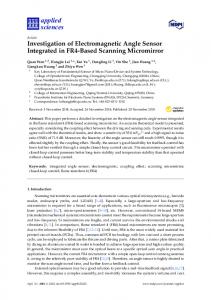
The study was conducted in an area irrigated with drainage waters in the Lower Seyhan Plain (213 000 ha) on the southern coastal Mediterranean region near Adana, Turkey, where irrigation has increased since 1960 to cover 133 431 ha in 2002 [28], or about 10% of the total irrigated area in Turkey (Figure 1). The 7 110 ha Yemisli Irrigation District, located in the Fourth Stage Project Area, with a mean altitude of 2.37 meters above mean sea level (range of 0.97 to 6.28 m), is one of the most productive agricultural areas. The District has limited fresh water resources due to incomplete irrigation infrastructures; therefore, farmers are dependent on drainage waters with EC values of 1.2 to 4.0 dS m-1. In addition, low soil permeability, high soil salinity and shallow and high saline (EC ≥15 dS m-1) groundwaters are the main constraints. However, open-sur-face drainage ditches have been constructed and the main irrigation canals are in progress. The main drainage ditches, carrying irrigation-tail waters and up-stream drainage waters, cut across the Project area and discharge into the Mediterranean Sea. The District geographically lies between 36o 36′ 11′′ and 36o 43′ 40′′ N latitude, and 35o 20′ 08′′ and 35o 27′ 40′′ E longitude. The area has a Mediterranean-type climate, typically with hot and dry summers, and mild and rainy winters [29]. Rainfall mainly occurs during winter months, with minimum evaporation, showing an inverse relationship between temperature and rainfall, and therefore evapotranspiration (Figure 2). Mean annual rainfall is considerably higher than most areas of the Mediterranean basin, i.e., 766 mm, with only 15% of that amount falling between April and September and most (54%) occurring in November to January, the wettest period. Long-term mean, maximum and minimum monthly temperatures for the period 1964-2008 are 18.9, 27.9 and 10.0 ºC, respectively (data taken from Karatas meteorological station of State Meteorological

1134



Black Sea

Aegean Sea

Ankara Iran

TURKEY Antalya

Adana Iraq Syria

Mediterranean

FIGURE 1 - Location of the Lower Seyhan Plain (LSP) in Turkey and Yemisli Irrigation District (YID)

300

900 Long-term means 2008 Cumulative

200 Rainfall (mm)

700

Irrigation season (May 20 - August 15)

600 500

150 400 100

300

200 50

Cumulative mean rainfall inthe long term (mm)

800

2007 250

100

Ju ne

ay M

A pr il

ar ch M

ry

ry

Fe br ua

nu a Ja

em be r

D ec

be r

er

em N ov

ct ob O

Se p

te m

be r

t

0

A ug us

Ju ly

0

Months

FIGURE 2 - Temporal variability of long-term monthly mean rainfall (CV=85%) and year-to-year variability of monthly rainfall in 2007 and 2008. Vertical bars indicate ±1 standard error of the long-term means

1135



Affairs, about 8 km from the District). Highest mean temperatures occur in August (280C) and lowest in January (100C). Soil moisture and temperature regimes in the District are xeric and thermic, respectively, based on the climatic data of the study area. The soils (Figure 3) are mainly formed on “aged river terraces” and “delta base” and are classified as Entisols, i.e., Aquic Xerofluvent (Arpaci Series, 23%) and Inceptisols, i.e., Vertic Haplaquept (Helvaci Series, 50%), respectively [30]. The soils are generally deep and high in clay and calcium carbonate. Variation in the distribution of soil properties in the District, especially texture, is a factor impinging on the distribution of salinity and the degree of drainage. The cropping pattern is mainly wheat (Triticum aestivum), barley (Hordeum vulgare), and cotton (Gossypium hirsutum), which is relatively salttolerant, and to lesser extent, corn (Zea mays), citrus and melons (Citrullus vulgaris) that are cultivated in the northern part of the District, where neither soil salinity nor shallow groundwaters are a significant problem.

2.2. Sampling for Soil Salinity Assessment

Groundwater salinity and depth observations, and ECa data were recorded and processed for the 2007 and 2008 hydrological years (October 1 to September 30 of the following year). Four sets of ECa readings were recorded in 2007 (March, June, July, October) and 2008 (February, April, July, September) in the horizontal (for 0-1 m soil layer) and vertical (for 0-2 m soil layer) dipole-mode configurations using a hand-held EM38 device integrated with a GPS. Concurrently with ECa readings, soil temperatures at the same sites were measured at 0.5 m and 1.0 m soil depths for the horizontal and vertical dipole-mode readings, respectively, to adjust ECa readings to a reference temperature of 25 °C. The locations of the EM38 readings were selected randomly over the entire area. The number of geo-referenced ECa reading sites varied from 97 to 145 at each sampling time, depending on the accessibility to the sampling sites in the field. The existing 56 groundwater observation wells (Figure 4) served as a benchmark in the field, and measurements were always recorded as close

FIGURE 3 - Soil series distribution in the Yemisli Irrigation District (adapted from Dinç et al. [30])

1136



as possible to the observation wells at each sampling. Repeated measurements in time were recorded at the same sites using the GPS device. A sketch of the District (Figure 4) shows the observation wells, the soil sampling points for EM38 calibration, the primary and secondary drainage canals, and the locations of groundwater level recorders and freshwater diversion points, if applicable. The entire study area and the full range of totally 53 EM38 readings (33 in March 2007 and 20 in February 2008) were selected for soil sampling and ECe determinations that were used for calibration of the EM38 sensor. For this purpose, the soil samples (Figure 4) were collected just beneath the sites where the EM38 measurements were made using a hand-auger over 0-2.0 m depth with 0.3 m depth increments [31]. The soil samples from 0-0.3, 0.30.6, 0.6-1.0, 1.0-1.3, 1.3-1.6, 1.6-2.0 m soil depth increments were air-dried, ground and sieved, and composite

samples were prepared to measure the average ECe for the 0-1 m and 0-2 m soil depths using the procedure given in Richards [32]. Because the EC readings are temperaturesensitive [17], they were adjusted to a reference temperature of 25 °C using the following relation (Eq. 1) given in Richards [32].

EC 25 = ft EC t ft = 0.4470 + 1.4034 e −t / 26.815

(1)

where ECt and ft stand for the electrical conductivity readings made at a particular temperature t and temperature correction factor, respectively. The ECa readings, adjusted to 25 °C, were converted into ECe estimates using the calibration equations developed for the study site. These ECe estimates were then used to construct the soil salinity maps using GIS tools [20].

FIGURE 4 - Groundwater observation wells and irrigation water diversion sites with the main drainage network in the Yemisli Irrigation District

1137



2.3. Mapping Spatial and Temporal Variability of Soil Salinity

Maps of ECe for the two soil depths at each survey were developed using ArcView 3.0a GIS [33], which is considered a useful tool to organize, manipulate, and display complex spatial data such as soil salinity [34]. For the mapping procedure, the point themes were generated through the use of geo-referenced ECa readings. The ESAP software [35] allows for inverse-distance-squared weighted interpolation technique in assessing, predicting and mapping soil salinity in irrigated areas. The inverse-distance-weighted (IDW) interpolation determines grid-cell values using a linearly weighted combination of a set of sample points (Eq. 2). The weights are determined as a function of inverse distance to a power β. The surface being interpolated should be that of a spatially correlated variable [36]. Details of the IDW algorithm, as applied to each location where an estimation is made, can be found in Tomczak [37] and Cetin and Diker [38]. The general prediction equation is given as n

zˆ0 = ∑ i =1

1 n

(hi 0 ) ∑ (hi 0 ) β

−β

zi

(2)

i =1

where

zˆ0

is the interpolated value of the cell con-

sidered, Zi are the neighbouring data points, hio are the Euclidean distance between the cell centre and data points used in the interpolation, β is the power, and n is the

number of neighbouring data points used in the interpolation procedure. In this study, interpolations were carried out using n=12 and β=2, and cell size for the interpolation technique was fixed to 50 m by 50 m. Zonal statistics as well as histograms of the maps produced in GIS media were used to develop both areal mean soil salinity over the study area for the average soil profiles (i.e. 0-1 and 0-2 m), and hypsometric soil salinity curves [27] for comparing the maps obtained at different sampling times. Likewise, we estimated ECe data at unvisited locations using this technique. 3. RESULTS 3.1. Soil Data Analysis and ECa-ECe Calibration

A summary of the 2007 and 2008 ECe data measured at specific points for developing the District-specific ECaECe calibration equations, along with statistical parameters, is presented in Table 1. Although the mean ECe in the upper soil (0-0.3 m) was lower than the ECe value of 4 dS m-1 that classifies the soils as being saline [32], the maximum ECe encountered was over 16 dS m-1, which is highly saline. The range between maximum and minimum ECe values was reflected in a high coefficient of variation. The mean, median and coefficient of skewness of the data obtained with depth suggest that soil profile salinity was not normally distributed. However, the logarithmic transformation did not improve the calibration curves for both

TABLE 1 - Descriptive statistics of ECe for three soil sampling depths, temperature adjusted ECa readings, 0-1 m composite ECe, and 0-1 m predicted ECe from the ECa readings and the ECa-ECe calibration equations

Statistics Mean Standard error of mean Median Standard deviation Kurtosis Skewness Minimum Maximum Number of sites sampled Confidence Level (95.0%) Coefficient of Variation (%) Mean Standard error of the mean Median Standard deviation Kurtosis Skewness Minimum Maximum Number of sites sampled Confidence Level (95.0%) Coefficient of Variation (%)

0-0.3 m

ECe 0.3-0.6 m

2007 (Mar)

3.9 1.0 1.5 5.7 5.3 2.3 0.3 24.9 33 2.0 144

5.3 1.2 1.8 7.0 2.9 1.9 0.5 25.7 33 2.5 131

2008 (Feb)

2.9 0.8 1.4 3.7 7.8 2.6 0.4 16.1 20 1.8 128

5.2 1.4 3.0 6.2 1.3 1.5 0.4 19.9 20 2.9 119

Year

1138

ECa 0.6-1.0 m 0-1 m dS m-1 7.0 2.8 1.5 0.4 3.3 2.0 8.8 2.2 4.2 1.8 2.1 1.6 0.7 0.8 37.8 8.7 33 33 3.1 0.8 125 78 7.7 1.8 4.9 7.9 0.7 1.4 0.4 25.5 20 3.7 102

3.0 0.5 2.2 2.4 2.6 1.7 0.4 9.8 20 1.1 82

Composite ECe Predicted ECe 0-1 m 5.7 1.2 2.5 7.0 2.9 1.9 0.5 27.7 33 2.5 123

5.8 1.2 3.1 6.8 3.4 2.1 1.0 26.3 33 2.4 117

5.8 1.6 3.4 7.4 4.9 2.2 0.4 29.1 20 3.4 126

5.9 1.6 3.3 7.2 5.6 2.4 0.5 29.0 20 3.4 122



soil depths in either year. Soil salinities for three soil depths and the bulk profile of 0-1 m had a right-skewed distribution. Such a distribution may be attributed to successive random dilutions [39], mostly contributed by flat topography, micro-relief, poor quality groundwater, and soil salinity increases with depth. Mean composite ECe values for soil-sampling sites were almost the same (5.7 dS m-1 in 2007 and 5.8 dS m-1 in 2008), indicating salinity persistence in the District. At the end of the wet season (March), mean salinity distribution in the profile was normal, (i.e., ECe values increasing with depth), indicating a leaching effect of winter rains. The Pearson product moment correlation coefficients between composite soil ECe for 0-1 depth and ECa data were highly significant (P20 dS m-1, compared to the groundwater depths observed in each year. Because the water table was close to the soil surface in the wet season, winter rains remained within the root zone and in the depression areas, preventing saline groundwater capillary rise. However,

means of ECe over the 0-1 m soil profile were inherently higher than 4 dS m-1 in successive years (Figure 5), exhibiting moderate soil salinity within the root zone just after the completion of winter rains. Calibration equations were developed separately for the 0-1 m and 0-2 m soil depths in 2007 and 2008. Parameters and statistics of the quadratic type calibration equations were presented in Table 2 where the R2 values of the calibration equations for the two depths for both years were high (R2>0.95) and statistically significant (p< 0.05). Thus, calibration equations accounted for over 95% of spatial variation [40] of the observed soil salinity. Although model coefficients are not just the same for each depth in 2007 and 2008, determination coefficients are nearly the same (Table 2), and standard error of the models are around “one”. As an example, Figure 6 shows visually the calibration equation for the 0-1 m soil depth. Composite soil salinities (ECe) obtained in the laboratory and predicted soil salinity (ECe) values by calibration equations showed nearly a linear (1:1) relationship. As pointed out by de Jong et al. [21], this type of relationship is an indication of representativeness of the calibration equations. 3.1.1. Preliminary Exploration of EM38 data

Table 3 gives the descriptive statistics of the ECe estimates obtained from the ECa readings and the calibration equations at the different survey dates in 2007 and 2008 (Table 2). ECe showed spatial and temporal vari-1

Salinity (ECe, dS m )

2

4

6

8

0 30

Depth (cm)

60 90 120 150 180

Mean ECe in March/2007 Mean ECe in 0-1 depth in March/2007 Mean ECe in Feb/2008 Mean ECe in 0-1 depth in Feb/2008

FIGURE 5 - ECe profiles obtained in the Yemisli Irrigation District in 2007 and 2008

TABLE 2 - ECe=a ECa2+b ECa type calibration model parameters for 0-1 m and 0-2 m soil depths in March 2007 and Feb. 2008 0-1 m soil depth Model parameters a b Determination coefficient (R2) Standard error of the model (Se) Number of observations

2007 0.219 1.010 0.976 1.119 33

0-2 m soil depth 2008 0.207 1.030 0.975 1.188 20

1139

2007 0.163 0.871 0.958 1.148 33

2008 0.192 0.884 0.982 0.981 20



30 ECe 0-1 m = 0.1965 ECa

2 t 0-1 m+

1.0323 ECat 0-1 m

2

ECe, dS m

-1

R = 0.9753

20

10

EM38 Calibration (0-100 cm)

0 0

2

4

6

8

10

12

-1

ECat, dS m

FIGURE 6 - Relationship and calibration equation between ECa readings in the horizontal dipole position and 0-1 m depth mean ECe in year 2008

TABLE 3 - Descriptive statistics of ECe (dS m-1) estimates for the 0-1 and 0-2 m soil depths obtained at each 2007 and 2008 survey dates 0-1 m soil depth

0-2 m soil depth dS m-1

Statistics Mean Standard error of the mean Median Standard deviation Kurtosis coefficient Skewness coefficient Range Minimum Maximum Number of sites sampled Confidence Level (95.0%) Coefficient of variation (%)

Mean Standard error of the mean, SE Median Standard deviation, SD Kurtosis coefficient, Ck Skewness coefficient, Cs Range Minimum Maximum Number of sites sampled, n Confidence Level (95.0%) Coefficient of variation (%)

Year

2007

2008

March 7.2 0.9 3.3 10.3 8.5 2.8 54.1 0.5 54.6 124 1.8 143

June 3.6 0.4 2.5 3.6 9.2 2.6 22.4 0.4 22.8 97 0.7 99

July 4.4 0.5 2.7 4.9 12.0 3.0 32.1 0.5 32.5 103 1.0 109

Oct. 3.6 0.6 1.7 6.4 27.7 4.9 44.2 0.2 44.5 106.00 1.2 180

March 7.7 0.8 4.4 9.0 7.1 2.4 54.0 0.4 54.4 124.00 1.6 116

June 5.0 0.5 3.1 5.2 3.8 1.8 25.5 0.3 25.8 97 1.0 104

July 6.3 0.7 3.8 6.9 9.8 2.6 45.3 0.3 45.6 103 1.4 109

Oct. 5.4 0.8 2.5 8.0 18.0 3.8 55.7 0.3 56.0 106 1.5 149

Feb. 4.9 0.6 2.5 6.0 15.1 3.3 41.7 0.5 42.1 112 1.1 122

April 4.2 0.4 2.3 4.3 5.8 2.2 25.0 0.2 25.2 145 0.7 103

July 3.5 0.3 2.4 3.6 16.4 3.3 27.3 0.3 27.6 138 0.6 103

Sep. 3.5 0.3 2.0 3.5 4.3 2.0 18.7 0.1 18.8 106.00 0.7 102

Feb. 5.9 0.6 3.5 6.3 8.5 2.5 39.5 0.6 40.0 112.00 1.2 106

April 5.4 0.4 3.3 5.2 3.6 1.8 26.9 0.2 27.1 145 0.9 96

July 4.9 0.4 3.4 4.6 8.3 2.4 31.0 0.4 31.4 138 0. 8 95

Sep. 4.4 0.4 2.7 4.3 3.3 1.8 21.3 0.2 21.5 106 0.8 98

ability between and within years in the irrigation District. Differences between minimum and maximum ECe in any survey were always over 18 dS m-1. ECe and its spatial

variability increased with soil depth, indicating normal salinity profiles. The medians were lower than the means, indicating a right-skewed ECe distribution due mainly to

1140



different cropping systems and agricultural practices [20], low topography and poor management conditions. Skewness coefficients were high and positive for the two soil depths and sampling dates in both years, again indicating a significant deviation of ECe from normality. Regardless of soil depth (0-1 or 0-2 m), ECe estimates were consistently highest in March 2007, with small differences between the other months (June, July and October). However, ECe tended to be higher in the 0-2 m than in the 0-1 m depth soil profile. This variability and the higher ECe in 2007 than in 2008 is most probably due to a more homogenous distribution of rainfall in 2008 (Figure 2), although it was 20% lower than in 2007. 3.2. Mapping Spatial and Temporal Variability of Soil Salinity (ECe)

The spatial and temporal variability of ECe is given in Figure 7 before (March) and at the end (October) of the irrigation season. As both years showed the same spatial distribution patterns, only the 2007 maps are shown. The highest salinity areas (darker zones) were present in the south, whereas the non-saline areas dominated the northwest of the study area in the rainy periods. Contrary to expectations, the low salinity areas expanded in the driest

period (September or early October), even though saline drainage waters were used for irrigation. This was attributed to fresh water being diverted from IW1 that was available for irrigation along the YS6 canal (Figures 4, 7). The ECe values at 0-2 m soil depth showed a similar spatial distribution pattern, although it was higher than ECe at 0-1 m soil depth. Hypsometric ECe curves (Figure 8), based on tabulated values of the ECe map histograms for the two soil depths, provide an indication of soil salinity extent. The areal extent of root zone (0-1 m) ECe was the same in July (peak irrigation season) and late September (Figure 8) indicating that a leaching regime prevailed in the area during the irrigation season despite the use of saline drainage waters. The 2007 and 2008 hypsometric ECe curves were nearly similar. The salinity reductions between the wet and dry periods were higher at 0-1 m than at 0-2 m soil depths (Figure 8). Similar results were obtained by Benyamini et al. [41]. Hypsometric salinity curves allow us to conclude that at least one-third of the study area has persistent salinity problem (ECe>4 dS m-1) in the monitoring period.

a) March 2007/ 0-1 m

b) Early October 2007/ 0-1 m

FIGURE 7 - Spatial and temporal variability of the estimated ECe for 0-1 m depth in the Yemisli Irrigation District in the hydrological year 2007

1141



FIGURE 8 - Hypsometric ECe curves for the (a) 0-1 m and (b) 0-2 m soil depths in hydrological year 2008. Two-sided arrow and horizontal dotted line indicate the salinity reduction in the period considered and threshold level of soil salinity, respectively

4. DISCUSSION This study in an irrigated area of southern Turkey highlighted the issue of secondary salinity as influenced by the management practices, especially when poor quality drainage water is used for irrigation purposes. Thus, it adds to a growing body of research on irrigation in the Mediterranean region [18], where soil salinization is a major issue. The factors dictating salt balance in irrigated soils are evaporative demand under arid and semi-arid conditions, and inadequate removal of salts from the root zone due to poor drainage, in essence, the leaching regime [13]. The high clay content [30], dominated by smectite-type minerals, has likely contributed to poor drainage, as was also previously noted for the same area by Cetin and Kirda [27], where irrigation water is relatively high in salts and the issue of leaching is critical.

As spatial variability is an inherent characteristic of soils, compounded by variation in landscape topography, any large-scale irrigated area is bound to exhibit wide variations in soil salinity. Consequently, in the Yemisli Irrigation District relatively small variations in elevation probably contributed to considerable salinity variations over the entire irrigated area (Figure 7), though no correlations were made between elevation and salinity due to scanty elevation data of high resolution. Indeed, in some low-lying areas with poor drainage outlets, there may be lateral movement of salts which could contribute to the spatial variability of salinity [42]. With respect to salinity management, the issue is how salinity changes temporally within and in between seasons. Some farmers have no options other than using the provided available water, whether it is poor quality groundwater or drainage water such as the similar source used in the Yemisli District. However, farmers and local water ma-

1142



nagers have some options for mitigating the effects of secondary salinity buildup. Installation of a drainage system to lower the water table is the most obvious one in the district. The groundwater level should be kept below 1 m from the surface depending on some soil factors, especially soil texture [41]. Ultimately, such drainage infrastructures will be in place as the Yemisli Project is further developed. Even so, the success of the system will still be questionable, because the required pumping drainage is much more expensive than the gravitational drainage, and is essential in this and other low-lying areas within the Mediterranean region. The rationale in the Yemisli District for using poor quality waters for irrigation in a system without proper drainage facilities is the salinity control by synchronizing irrigation in the dry summer following the wet winter and spring seasons of a typical Mediterranean climate [29]. Thus, any salinity buildup in the dry summer season is believed to be flushed out of the root zone following the rainy season. The seasonal ECe data in our two years study did not suggest any substantial increase in salinity within and between years. In fact, a detailed study of a 0.27 ha cotton field in the Yemisli District [27] showed that the existing irrigation practices in the summer months (June to August) did not increase soil salinity. However, this conclusion is necessarily limited, since valid conclusions require a long-term perspective on irrigation practices. This perspective requires soil salinity monitoring in time and space, implicitly raising the question of how effectively and economically such monitoring can be done. The findings of this study offer a potential solution to large-scale salinity monitoring. Soil salinity measurement [43] is not a viable option because of the relative scarcity and shortcomings of public and private laboratories for such analysis in the Mediterranean region [44], as well as questionable quality control in the analyses themselves [45]. The use of electromagnetic induction sensors, such as the EM38, has shown to be an effective alternative for assessing soil salinity in time and space [14, 18, 46]. Hence, the actual electromagnetic readings can be readily converted to ECe estimates [20, 21], provided that on-site calibration is done for the intended irrigation scheme being monitored. In principle, to estimate ECe in the study area, the EM38 device must be calibrated within the study area, and at the time of measurements [31]. In this study, calibration equations were developed in two successive years. ECa-ECe relationship is generally expected to be linear. As seen in Table 2, our calibration equations are in the quadratic form, though quadratic type regression equations are rarely observed in salinity studies [40]. Even so, the developed calibration curves satisfactorily predicted ECe from the acquired EM38 data at a particular date. Soil salinity, clay content, cation exchange capacity, poresize distribution, soil moisture content and temperature all affect ECa [18]. The relationship between ECa and ECe led us to conclude that the EM38 sensor can be calibrated as a direct measurement of soil salinity that is the most

dominant factor in the District. Although, the model coefficients are not just the same for each depth in 2007 and 2008, determination coefficients are nearly the same (Table 2), and the standard errors of the models are around “one”. A number of factors such as errors made in the laboratory, soil moisture content, spatial variability of soil physical and chemical characteristics etc. may have influences on the regression coefficients of calibration equations. Therefore, it might be expected to have different regression constants even though negligible. Accordingly, one of these equations developed can be used in salinity surveys in the study area. A study by Diaz and Herrero [31] suggested that the calibration equation developed at one date could be used reliably to predict the salinity for the study area from EM38 measurements taken at another date. In our study in the Yemisli Irrigation District, the EM38 device proved to reliably and quickly map soil salinity, following the appropriate calibration. This device can further be adapted to other irrigation schemes within Turkey or other Mediterranean-irrigation districts [18]. Incorporating EM38 data with GIS enabled us to drive further information on the severity and extent of soil salinity. 4. CONCLUSIONS This two-year study of a large-scale irrigation Project in southern Turkey irrigated with poor quality drainage waters showed that soil salinity can be easily and reliably monitored using the EM38 electromagnetic induction device. While there was little evidence to show that salinity was exacerbated within the limited 2-year time-frame considered, the salinity maps and the associated hypsometric salinity curves are strategies that can be used for the longterm monitoring of irrigation projects. ACKNOWLEDGMENTS Authors gratefully acknowledge that this work was funded by the European Union in the context of FP6 with project acronym QUALIWATER (Project #: INCO-CT2005-015031) and partial support received from Cukurova University Research Projects Unit (Project #: ZF2006KAP1 and ZF2009KAP1).

1143

REFERENCES [1]

Godfray, H.C.J, Beddington, J.R., Crute, I.R., Haddad, L., Lawrence, D., Muir, J.F., Pretty, J., Robinson, S., Thomas, S.M. and Toulmin, C. (2010) Food security: the challenge of feeding 9 billion people. Science, 327 (5967): 812-818.

[2]

Federoff, N.V., Battisti, D.S., Beachy, R.N., Cooper, P.J.M., Fischhoff, D.A. and Hodges, C.N., Knauf, V.C., Lobell, D., Mazur, B.J., Molden, D., Reynolds, M.P., Ronald, P.C., Rosegrant, M.W., Sanchez, P.A., Vonshak, A. and Zhu, J.-K. (2010) Radically rethinking agriculture for the 21st century. Science, 327 (5967): 833–834.



[3]

Rosegrant, M.W., Cai, X. and Cline, S.A. (2002) World water and food to 2025: dealing with scarcity. International Food Policy Research Institute, Washington, DC, USA, 322 pp.

[4]

Doll, P. and Siebert, S. (2002) Global modeling of irrigation water requirements. Water Resources Research, 38: 10371037.

[5]

Boutraa, T. (2010) Improvement of water use efficiency in irrigated agriculture: A review. Journal of Agronomy, 9: 1-8.

[6]

Hussain, I. (2007) Direct and indirect benefits and potential disbenefits of irrigation: evidence and lessons. Irrigation and Drainage, 56: 179-194.

[7]

Bhutta, M.N. and Smedema, L.K. (2007) One hundred years of waterlogging and salinity control in the Indus Valley, Pakistan: a historical review. Irrigation and Drainage, 56: S81-S90.

[8]

Singh, A., Krause, P., Panda, S.N. and Flugel W.-A. (2010) Rising water table: A threat to sustainable agriculture in an irrigated semi-arid region of Haryana, India. Agricultural Water Management, 97: 1443-1451.

[9]

Gopalakrishnan, M. and Kulkarni, S.A. (2007) Agricultural land drainage in India. Irrigation and Drainage, 56: S59-S67.

[10] Lal, R. and Stewart, B.A. (1990) Soil degradation: A global threat. Advances in Soil Science, 11: 13-17. [11] Aragüés, R. and Tanji, K.K. (2003) Water Quality of Irrigation Return Flows. In: Stewart B.A. and Howell, T.A. (eds) Encyclopaedia of Water Science, Marcel Dekker Inc., New York, 502-506 pp. [12] Selle, B., Thayalakumaran, T. and Morris, M. (2010) Understanding salt mobilization from an irrigated catchment in south-eastern Australia. Hydrological Processes, 24: 33073321. [13] Letey, J., Hoffman, G.J., Hopmans, J.W., Grattan, S.R., Suarez, D., Corwin, D.L., Oster, J.D., Wu, L. and Amrhein, C. (2011) Evaluation of soil salinity leaching requirement guidelines. Agricultural Water Management, 98: 502-506. [14] Herrero, J., Ba, A.A. and Aragüés, R. (2003) Soil salinity and its distribution determined by soil sampling and electromagnetic techniques. Soil Use and Management, 19: 119-126. [15] Amezketa, E. (2007) Soil salinity assessment using directed soil sampling from a geophysical survey with electromagnetic technology: a case study. Spanish Journal of Agricultural Research, 5 (1): 91–101. [16] Rongjiang, Y. and Jingsong, Y. (2010) Quantitative evaluation of soil salinity and its spatial distribution using electromagnetic induction method. Agricultural Water Management, 97: 1961-1970. [17] Smedema, L.K., Vlotman, W.F. and Rycroft, D.W. (2004) Modern Land Drainage: Planning, Design and Management of Agricultural Drainage Systems. A.A. Balkema Publishers, London, UK, 447 pp. [18] Aragüés, R., Urdanoz, V., Cetin, M., Kirda, C., Daghari, H., Ltifi, W., Lahlou, M. and Douaik, A. (2011) Soil salinity related to physical soil characteristics and irrigation management in four Mediterranean irrigation districts. Agricultural Water Management, 98: 959–966. [19] FAO (2001) Drainage and Sustainability. IPTRID Issues Paper, No. 3, Food and Agriculture Organization of the United Nations, Rome, Italy.

1144

[20] Corwin, D.L. and Lesch, S.M. (2005) Apparent soil electrical conductivity measurements in agriculture. Computers and Electronics in Agriculture, 46: 11-43. [21] de Jong, E., Ballantyne, A.K., Cameron, D.R. and Read, D.W.L. (1979) Measurement of apparent electrical conductivity of soils by an electromagnetic induction probe to aid salinity surveys. Soil Science Society of America Journal, 43 (4): 810-812. [22] Harlan, J.R. (1992) Crops and Man. American Society of Agronomy, 677 S. Segoe Road, Madison, WI 53711, 284 pp. [23] Khouri, N., Shideed, K. and Kherallah, M. (2011) Food security: Perspectives from the Arab World. Food Security, 3 (Suppl. 1): S1-S6. [24] El-Fadel, M., El-Sayegh, Y., Abou, I.A, Jamali, D. and ElFadl, K. (2002) The Euphrates-Tigris basin: A case study in surface water conflict resolution. Journal of Natural Resources and Life Sciences Education, 31: 99-110. [25] Ibrikci, H., Cetin, M., Karnez, E., Topcu, S., Kirda, C., Ryan, J., Oguz, H., Dingil, M. and Oztekin, E. (2010) Monitoring groundwater nitrate concentrations under irrigation in the Cukurova region of southern Turkey. Fresenius Environmental Bulletin, 19 (9): 1802-1812. [26] Ibrikci, H., Cetin, M., Karnez, E., Kirda, C., Topcu, S., Ryan, J., Oztekin, E., Dingil, M., Korkmaz, K. and Oguz, H. (2012) Spatial and temporal variability of groundwater nitrate concentrations in irrigated Mediterranean agriculture. Communications in Soil Science and Plant Analysis, 43:47-59. [27] Cetin, M. and Kirda, C. (2003) Spatial and temporal changes of soil salinity in a cotton field irrigated with low-quality water. Journal of Hydrology, 272: 238-249. [28] Cetin, M., Kirda, C., Efe, H. and Topcu, S. (2007) Using geographic information system for investigating soil and groundwater salinity caused by using low quality irrigation water. (in Turkish with English abstract) Presented orally in the Second Conference on Water Politics organized by Turkish Chamber of Architectures and Engineers, Conference Proceedings Book, 20-22 March 2008, Ankara, Turkey, pp. 471-481. [29] Kassam, A.H. (1981) Climate, soil and land resources in the West Asia and North Africa Region. Plant and Soil, 58: 1-28. [30] Dinç, U., Sarı, M., Şenol, S., Kapur, S., Sayın, M., Derici, M., Çavuşgil, V., Gök, M., Aydın, M., Ekinci, H., Ağca, N. and Schlichting, E. (1995) Çukurova Bölgesi Toprakları. (in Turkish) Çukurova Üniversitesi Ziraat Fakültesi Yardımcı Ders Kitabı, No 26, Adana, Turkey. [31] Diaz, L. and Herrero, J. (1992) Salinity estimates in irrigated soils using electromagnetic induction. Soil Science, 154 (2): 151-157. [32] Richards, L.A. (Ed.) (1954) Diagnosis and Improvement of Saline and Alkali Soils. USDA Agricultural Handbook 60, Washington, DC, USA. [33] ESRI (1996) Using ArcView GIS. Environmental System Research Institute, Inc., Redlands, CA, USA. [34] Corwin, D.L. and Lesch, S.M. (2003) Application of soil electrical conductivity to precision agriculture: Theory, principles, and guidelines. Agronomy Journal, 95: 455-471. [35] Lesch, S.M., Rhoades, J.D. and Corwin, D.L. (2000) The ESAP-95 Version 2.01R User Manual and Tutorial Guide. Research Report No. 146. USDA-ARS, George E. Brown, Jr., Salinity Laboratory, Riverside, CA, USA.



[36] Keckler, D. (1995) SURFER® for Windows, Version 6, User's Guide. Golden Software, Golden, Colorado, USA, 511 pp. [37] Tomczak, M. (1998) Spatial interpolation and its uncertainty using automated anisotropic inverse distance weighting (IDW) – cross-validation/Jacknife approach. Journal of Geographic Information and Decision Analysis, 2: 18-33. [38] Cetin, M. and Diker, K. (2003) Assessing drainage problem areas by GIS: a case study in the Eastern Mediterranean Region of Turkey. Irrigation and Drainage, 52: 343–353. [39] Ott, W.R. (1995) Environmental Statistics and Data Analysis. Lewis Publishers, NY, 313 pp. [40] Sudduth, K.A., Kitchen, N.R., Bollero, G.A., Bullock, D.G. and Wiebold, W.J. (2003) Comparison of electromagnetic induction and direct sensing of soil electrical conductivity. Agronomy Journal, 95: 472-482. [41] Benyamini, Y., Mirlas, V., Marish, S., Gottesman, M., Fizik, E. and Agassi, M. (2005) A survey of soil salinity and groundwater level control systems in irrigated fields in the Jezre’el Valley, Israel. Agricultural Water Management, 76: 181-194. [42] Cetin, M. and Ozcan, H. (1999) Problems encountered in the irrigated and non-irrigated areas of the Lower Seyhan Plain and recommendations for solution: a case study. (in Turkish with English Abstract) Turkish Journal of Agriculture and Forestry, 23 (Suppl. 1): 207–217. [43] FAO (2002) Agricultural Drainage Water Management in Arid and Semi-Arid Areas. K.K. Tanji and N.C. Kielen (Eds.), Irrigation and Drainage Paper no 61, Food and Agriculture Organization, Rome, Italy, 204 pp. [44] Ryan, J. and Garabet, S. (1994) Soil test standardization in West Asia-North Africa. Communicationsin Soil Science and Plant Analysis, 25 (9&10): 1641–1655. [45] Ryan, J., Garabet, S., Rashid, A. and El Gharous, M. (1999) Soil laboratory standardization in the Mediterranean region. Communications in Soil Science and Plant Analysis, 30 (5&6): 885–894. [46] Amezketa, E. (2006) An integrated methodology for assessing soil salinization, a pre-condition for land desertification. Journal of Arid Environments, 67: 594–606.

Received: September 26, 2011 Revised: December 22, 2011 Accepted: January 19, 2012

CORRESPONDING AUTHOR Prof. Dr. Mahmut Cetin Department of Agricultural Structures and Irrigation Faculty of Agriculture University of Cukurova 01330 Balcali, Adana TURKEY Phone: +9053 3740 53 19 or ++90 (322)338 6877 Fax: ++90 (322) 338 6386 E-mail: [email protected] FEB/ Vol 21/ No 5/ 2012 – pages 1133 – 1145

1145