APPLIED PHYSICS LETTERS
VOLUME 77, NUMBER 10
4 SEPTEMBER 2000
Imaging soft samples in liquid with tuning fork based shear force microscopy W. H. J. Rensena) and N. F. van Hulst Applied Optics Group, University of Twente, P.O. Box 217, 7500 AE Enschede, The Netherlands
S. B. Ka¨mmer ThermoMicroscopes, 1171 Borregas Avenue, Sunnyvale, California 94089
共Received 5 May 2000; accepted for publication 17 July 2000兲 We present a study of the dynamic behavior of tuning forks and the application of tuning fork based shear force microscopy on soft samples in liquid. A shift in resonance frequency and a recovery of the tip vibration amplitude have been observed upon immersion into liquid. Conservation of the vibration mode is confirmed by both direct stroboscopic observation and by detection of the tip vibration amplitude of the tuning fork. Thanks to the partial recovery of the Q factor upon complete immersion into liquid, it is possible to obtain high-resolution images on soft samples in liquid. This opens a new domain of applications for tuning fork based near-field scanning optical microscopes. © 2000 American Institute of Physics. 关S0003-6951共00兲04436-3兴
Tuning fork based shear force detection, as implemented in a large number of near-field scanning optical microscopes, has proven to be an easy and reliable method by which to control the distance between the probe and sample.1 Compared to optical shear force detection methods, the main advantages of tuning fork based shear force detection are the absence of elaborate optical beam alignment and interference between the near-field optical signal and the shear force detection optics. The application of near-field scanning optical microscopy 共NSOM兲 in biology requires the immersion of the sample and thus the probe in aqueous solution. Optical shear force and normal force detection schemes have already shown potential for imaging in liquids.2–4 A nonoptical method based on bulky piezo elements has also been demonstrated.5 Tuning fork based shear force detection is preferable, since tuning forks are small, sensitive, reliable, cheap force detectors.6 In principle, liquid immersion of the tuning fork can be avoided by immersing only the fiber tip.2,7 Such a method, however, requires some means of controlling the tip immersion depth into a liquid layer with micrometer stability. Although feasible, this complicates operation of the microscope and the exchange of fluids, making immersion of the whole tuning fork preferable. Until now, the huge damping of the tuning fork movement, occurring upon immersion into liquid, and a lack of understanding of the vibrational modes involved have prevented the use of tuning fork based shear force detection in liquids. In this letter we present the application of a tuning fork based shear force microscope on an annealed gold film and a cytospin sample, both in an aqueous environment. First, the common model describing the tuning fork dynamics is discussed. After that, the dynamic response of the tuning fork is investigated. The vibrational mode of the tuning fork is investigated by direct observation of the tuning fork movement a兲
Also at ThermoMicroscopes, 1171 Borregas Avenue, Sunnyvale, California 94089; electronic mail:
[email protected]
and by measuring the actual tip amplitude in air and water. Finally, the application of tuning forks for shear force microscopy in liquid environments is presented. The basic model for tuning fork dynamics was introduced by Karraı¨ and Grober.1 In their model, one prong of the tuning fork is modeled as a single beam that is allowed to bend in only one direction. This system behaves like a damped harmonic oscillator with an effective spring constant and an effective mass that can be calculated analytically. The damping is a fitting parameter to match the actual Q factor. The relative movement of the prongs, i.e., the interaction between the prongs and the potential movement in other directions, is not included in this model. The model is still valid if the prongs are moving like scissors, because then the base is practically fixed and the direction of movement follows the model. Yet, in practice many other vibrational modes are observed, each of them having a specific resonance frequency and a specific mode shape. Together they form an orthogonal set, i.e., any motion of the tuning fork can be explained as a superposition of vibrational modes. If an external dither piezo drives a tuning fork mechanically at various frequencies and the piezoelectric response of the tuning fork is recorded at each frequency, the dynamic response of the tuning fork is obtained. Multiple peaks that often show up in the dynamic response curve of the piezoelectric tuning fork signal indicate the presence of multiple modes. We have examined the dynamic response of 100 kHz tuning forks8 at increasing immersion depths in water. With a fiber attached to one of the prongs, the resonance frequency of the 100 kHz mode shifts, due to the increased mass and stiffness. While increased mass lowers the resonance frequency, higher stiffness increases the resonance frequency. Since the fibers are manually attached, the net effect varies slightly from tuning fork to tuning fork. Generally, a downshift of a few kHz is observed. The tuning fork is mechanically excited by an external dither piezo with a constant driving amplitude of the order of 10 pm. The driving frequency is swept from 78 to 98 kHz. A transimpedance amplifier amplifies the piezoelectric tuning fork signal and the ampli-
0003-6951/2000/77(10)/1557/3/$17.00 1557 © 2000 American Institute of Physics Downloaded 01 Sep 2003 to 130.89.25.109. Redistribution subject to AIP license or copyright, see http://ojps.aip.org/aplo/aplcr.jsp
1558
Appl. Phys. Lett., Vol. 77, No. 10, 4 September 2000
FIG. 1. Frequency sweeps of the piezoelectric tuning fork amplitude signal for increasing immersion depths. The curve up front is in air; the curve at the backside is for maximum immersion. The inset shows the vibration mode.
tude of the signal is recorded for each driving frequency. Figure 1 shows the dynamic response of one tuning fork for increasing immersion depths. The curve up front is obtained with the tuning fork in air while the curve at the back is obtained with the prongs completely immersed in water. The resonance frequency in air is close to 96.7 kHz with a high Q factor of about 1500. The next four curves correspond to increasing immersion of only the fiber tip, which results in a slight drop in resonance frequency and Q factor. As soon as the prongs touch the water surface, a meniscus builds up, resulting in a sudden drop in frequency and the Q factor for the sixth resonance curve. The frequency shift and the drop in the Q factor continue with further immersion of the tuning fork. With the prongs more than halfway immersed, the decrease in resonance frequency continues, however the Q factor starts to increase again to a value around 60. After complete immersion of the prongs, the resonance frequency stabilizes at 85.4 kHz and a Q factor of 62 and the fluid level is not critical anymore. The recovery of the Q factor and the shift in resonance frequency upon complete immersion raise the question of whether the tuning fork in water is moving in the same vibration mode as it is in air. We first have studied the behavior of the immersed tuning fork by direct observation. The tuning fork is mounted on a scanning probe microscope 共SPM兲 head9 that is placed on top of an inverted optical microscope to observe the underside of the two prongs. Their movement can easily be seen if the tuning fork is driven at high amplitude of ⬃10 nm. A light emitting diode, flashing at a few Hz off the driving frequency, is used as a strobe light to illuminate the tuning fork. At different driving frequencies, various modes are visible. At 96.7 kHz, the two prongs move towards and away from each other, as expected. The motion after immersion of the tuning fork is the same, however it is shifted to a resonance frequency of 85.4 kHz. We conclude that the tuning fork is oscillating in the same mode, both in air and in water at these two frequencies. Second, we have investigated the relation between the tip amplitude, or prong deflection of the tuning fork, and the driving amplitude of the dither piezo. A cleaved fiber, instead of a regular tapered fiber, is attached to the tuning fork for detection of the tip amplitude, resulting in a Q factor of 189. A red HeNe laser is coupled into the fiber and the scanner head is placed on top of the inverted optical microscope,
Rensen, van Hulst, and Ka¨mmer
FIG. 2. Tip amplitude vs driving amplitude for the tuning fork at resonance in air and in water. The Q factor is measured independently. The driving amplitude is calculated using the piezoelectric constant of the dither piezo 共0.3 nm/V兲. The tip amplitude scales with the Q factor.
with a position sensitive photodetector mounted to one of its output ports. With this detector, movements of the tuning fork prong from less than a nanometer to several microns can be detected.10 The detector was calibrated using the scanner in the SPM head. Figure 2 shows the results for tuning fork movement in air and water. The movement of the tuning fork is linear over a wide range of amplitudes. For small amplitudes, an offset of the amplitude is visible, resulting from noise in the measurement. The graph shows that, in water, the amplitude drops with the same factor as the Q factor does, as expected for a tuning fork in the same vibration mode. This result and the direct observation confirm that the tuning fork is moving in the same mode, at around 97 kHz in air and at 85 kHz in water. Having acquired knowledge that vibrational modes in water are similar to modes in air, where the forks can be successfully operated, tuning forks can be expected to work reliably in a liquid environment. A tuning fork that is completely immersed in water has a typical Q factor around 60 and is driven such that the tip amplitude is of the order of 1 nm. The phase of the piezoelectric tuning fork signal with respect to the drive is used as a measure for the tip–sample distance.10 With both prongs of the tuning fork fully immersed in water, the system is independent of the fluid level compared to other setups that are extremely sensitive to the immersion depth of the probe.2–5,7 To test the achievable resolution on a hard sample, an annealed gold surface is measured with the described setup. A drop of water, large enough to immerse the prongs completely, is deposited on the sample. In Fig. 3, different gold domains are clearly visible. The root mean square 共rms兲 ver-
FIG. 3. Topography of annealed gold in water, unfiltered, except for subtraction of a straight line at each scan line. The line frequency was 0.5 Hz; the rms noise in the image is 1.5 nm. Downloaded 01 Sep 2003 to 130.89.25.109. Redistribution subject to AIP license or copyright, see http://ojps.aip.org/aplo/aplcr.jsp
Rensen, van Hulst, and Ka¨mmer
Appl. Phys. Lett., Vol. 77, No. 10, 4 September 2000
FIG. 4. Topography on cytospin samples. All images show unfiltered data, except for subtraction of a straight line at each scan line. The Line frequency is 0.5 Hz. 共a兲 In air, the average height of the nucleus is 280 nm; the average height of the organelles is 160 nm above the glass. 共b兲 In water, the average height of the cell is 380 nm above the glass.
tical noise in this image is 1.5 nm over the area, obtained with a line frequency of 0.5 Hz. This result shows that with a tuning fork based setup high-resolution images can be obtained in water. Imaging of a relevant soft sample in water would prove sufficient sensitivity for future biological NSOM applications. To test whether this setup has low interaction forces and can handle soft biological samples, a cytospin sample was prepared. The topography of such a cytospin sample is first obtained using shear force detection with the sample in air. The cells on this sample are dried, so the membrane follows the solid remaining contents of the cell. This is visible in the topography, as shown in Fig. 4共a兲. The nucleus of the cell is clearly visible, as are several organelles. The av-
1559
erage height of the nucleus is 270 nm and the average height of the organelles is 160 nm above the glass. Immersing the sample into water may cause extreme damage to the cells, due to osmosis. Most cells fortunately showed a similar topography after being immersed in water and dried, indicating that these cells are not damaged by osmosis. The topography is obtained after placing a large enough drop of water onto the glass slide to immerse both prongs completely. Figure 4共b兲 shows the topography of a cell after immersion in water. This time, the organelles cannot be seen as clearly as in Fig. 4共a兲. The average height of the cell is 380 nm above the glass. We attribute this to absorption of water in the cell, which will raise the cell membrane. Apparently, the absorption is not strong enough to break the membrane. The topography of the cell can be repeatedly imaged without apparent damage to the cell. After drying, the topography becomes similar again to that in Fig. 4共a兲. Clearly, the interaction forces between tip and sample are small enough to prevent sample damage. In conclusion, we have demonstrated that a 100 kHz tuning fork can be used as a tip–sample distance detector in a liquid environment. Immersion experiments showed that complete immersion of both prongs of the tuning fork resulted in partial recovery of the Q factor. The vibrational mode of the tuning fork is conserved upon full immersion in water. The Q factor is determined by the dominant viscous damping in water and has a typical value of around 60. It is possible to obtain topography with good resolution and relatively low interaction forces with both prongs of the tuning fork immersed in water. Reproducible topographic images have been obtained on hard and soft samples. Currently we are incorporating a liquid cell in the setup in order to realize a near-field scanning optical microscope for biological applications, with a nonoptical, easy to use shear force height feedback system. The authors would like to thank Frans Segerink for the design and construction of the transimpedance amplifier. K. Karraı¨ and R. D. Grober, Appl. Phys. Lett. 66, 1842 共1995兲. P. Lambelet, M. Pfeffer, A. Sayah, and F. Marquis-Weible, Ultramicroscopy 71, 117 共1998兲. 3 P. J. Moyer and S. B. Ka¨mmer, Appl. Phys. Lett. 68, 3380 共1996兲. 4 C. E. Tally, M. A. Lee, and R. C. Dunn, Appl. Phys. Lett. 72, 2954 共1998兲. 5 R. Brunner, A. Bietsch, O. Hollricher, and O. Marti, Rev. Sci. Instrum. 68, 1769 共1997兲. 6 W. H. J. Rensen, N. F. van Hulst, A. G. T. Ruiter, and P. E. West, Appl. Phys. Lett. 75, 1640 共1999兲. 7 P. I. James, L. F. Garfias-Mesias, P. J. Moyer, and W. H. Smyrl, J. Electrochem. Soc. 145, L64 共1998兲. 8 ThermoMicroscopes model No. 1640-00. 9 ThermoMicroscopes Explorer. 10 A. G. T. Ruiter, K. O. van der Werf, J. A. Veerman, M. F. Garcia-Parajo, W. H. J. Rensen, and N. F. van Hulst, Ultramicroscopy 71, 149 共1998兲. 1 2
Downloaded 01 Sep 2003 to 130.89.25.109. Redistribution subject to AIP license or copyright, see http://ojps.aip.org/aplo/aplcr.jsp