In this report we describe a method for extracting curves from an image using directional pixel variances instead of gradient measures as low-level boundary ...
Using directional variance to extract curves in images, thus improving object recognition in clutter � Andrea Selinger and Randal C. Nelson Department of Computer Science University of Rochester Rochester, NY 14627 (selinger, nelson)@cs.rochester.edu
Abstract
In this report we describe a method for extracting curves from an image using directional pixel variances instead of gradient measures as low-level boundary evidence. The advantage of the variance over the image gradient is that we can accurately compute the direction of a local edge even if a sudden contrast change occurs in the background. This allows curves belonging to object contours to be followed more easily. We compared our method to a similar method based on the image gradient and we found that it obtains better results when run on synthetic and natural images. Our method also improved the performance of a contour-based 3D object recognition system in cluttered images. Key Words: edge detection, boundary extraction, 3D object recognition.
�
Support for this work was provided by ONR grant N00014-93-I-0221, and NSF IIP Grant CDA-94-01142
1
1 Introduction Finding curves in an image is an important step in many object recognition and scene analysis applications. The most widely used methods are based on linking edge pixels that are extracted from the image using some low-level process. Well known and widely used edgel extraction methods are the ones developed by Canny [7] and Marr and Hildreth [9]. Several methods have been used for edgel linking. One approach is to link edge pixels into contours on the basis of proximity and orientation. Examples include the Nevatia-Babu line detector [14], or the work of Zhou et al. [16], Nalwa and Pauchon [10], and Etemadi [3]. But these methods tend to be unstable in the presence of clutter, and have trouble bridging gaps. Some of these problems can be solved by using multiresolution representations [6] and grouping techniques [8]. Another method of curve detection is based on the Hough transform [2]. Here local edges vote for all possible lines they are consistent with, and the votes are summed up later to determine what lines are actually present. The disadvantages of this method are complexity, coarse resolution and lack of locality. The method developed by Burns et al. [1] partitions the image into a set of support regions based on the gradient direction. Each region will presumably be associated with a single feature. A method developed by Nelson [11] uses both gradient magnitude and direction information and incorporates explicit lineal and end-stop terms. These terms are combined nonlinearly to produce an energy landscape in which local minima correspond to lineal features. A hill climbing process is used to nd these minima. This method has signi cantly better gap-crossing characteristics than methods based on local edgel linking. The methods mentioned above, and most techniques in current use, utilize a local gradient measure to identify individual pixels (edgels) that may be involved in larger curves. The gradient has a serious drawback in the case of an object on a cluttered background that causes sudden contrast switches between the object and the background (such as a gray object placed on a checkerboard, see Figure 2). The gradient direction cannot be obtained accurately in the neighborhood of a contrast switch, so methods using the gradient direction have problems. The gradient magnitude also has a glitch in such a neighborhood, causing problems even for linking methods that don't use directional information at such points (which causes other ambiguities). Methods that don't use gradient direction at all obtain poor results in curve extraction in general. Grouping techniques can be a solution, but they might group together lines that are broken for other reasons. Another possibility is to use a facet model [5] to obtain an accurate estimate of the local boundary, but in the case of three planes meeting at a point (e.g., white, black and grey in Figure 2), the high number of parameters makes a solution in a small local neighborhood unreliable. Despite the problems with the gradient, both the existence and the direction of a continuous boundary across a contrast switch is unambiguous locally. As Fleck observes in [4], \boundaries demarcate objects in 3D space or distinctive regions in 2D camera images", hence a boundary is determined by the properties of one side. In other words, a boundary is essentially a one-sided object, and for a given point (for a given contour direction), there are two relevant \magnitudes". These correspond to evidence that the image is homogeneous 2
and di�erent from the other side on either side of the boundary. The problem with the gradient is that it lumps these distinct values into a single term. The problem manifests itself when one side of a boundary is homogeneous (corresponding to a single object) and the other is not. In this paper we describe a method that uses directional variances to locally assign two magnitudes and a direction to each potential edgel. A linking method similar to the one in [11] can then successfully extract contours of objects even in the case of a textured background with contrast changes. To demonstrate the improvement, the method is compared against a previously developed method [11] that uses an identical linking technique, but relies on a gradient-based measure of local boundary characteristics. We rst demonstrate that, for synthetic images of objects on contrast-reversing backgrounds, the new technique succeeds in extracting the desired boundaries, while the gradient-based method fails. We then demonstrate statistically, that for a large collection of natural images of objects on badly cluttered backgrounds, the new technique extracts more long boundary curves than the gradient-based method. The high-level comparison of di�erent curve extraction methods is a di�cult problem, since accepted objective empirical evaluation methodologies are still lacking. Shin et al. [15] suggested that a comparison method should evaluate an algorithm based on a vision task. To evaluate the system at this level, we chose the task of 3D object recognition, using the contour-based object recognition system described in [13] and [12]. We found that our variance based curve extraction method improved the performance of the system in the case of images of objects on cluttered backgrounds where silhouette information was crucial.
2 Method The edgel extraction method is based on the observation that the variance of pixels in a neighborhood of constant gray-scale or color (presumably coming from the same object) is much smaller than that of pixels in a neighborhood crossed by an edge. The changes in pixel variance allow us to estimate the magnitude as well as the direction of an edge. Edgels are then linked using a hill climbing method very similar to the one described in [11]. Our method extracts two local magnitudes for every edgel in the image. In the case of an object on a background, these can be considered as representing the local homogeneity of the object and the local homogeneity of the background. When a contrast change occurs in the background, the background boundary may break, but as long as the color of the object changes slowly, the object boundary evidence will be continuous, and can be locally linked. For object recognition, we are interested in the object boundary, the one that doesn't break as often. Hence for the recognition test we discard curves that are subsumed by longer curves (i.e. curves belonging to the background boundary are discarded).
2.1 Extracting edgels using directional variance
What we refer to as \edgel extraction" in the following is not a simple \threshold" process where a binary decision is made as to whether the pixel lies on a boundary or not. Rather the term refers to the process of assigning a direction and two magnitudes to each pixel, where 3
Figure 1: Points used in variance computation for three directions; the potential edge pixel is marked with an x the direction indicates the best boundary direction, and the two magnitudes re ect the evidence that there is a transition to a distinct, homogeneous region crossing the boundary in either direction. Before starting the edgel extraction process, we perform a 3x3 median ltering on the image to eliminate shot noise, which can negatively impact variance measures. We then smooth the image with a circular Gaussian lter having a half-width at half maximum of 1 pixel (standard deviation = 1.18 pixels) in order to eliminate aliasing e�ects that might arise in a synthetically generated or point-sampled image. To evaluate the evidence that a pixel lies on a boundary we need to compare the variances of di�erent groups of pixels in the neighborhood of our pixel. We compute a symmetric variance vsym for a 3x3 neighborhood about the pixel, and 16 directional variances v� corresponding to short, o�set linear regions in di�erent directions from the central pixel (every 22.5 degrees). Speci cally, for each angle (potential edge direction) we step one pixel away in the direction perpendicular to that angle. This is the minimum distance to avoid a grid aliasing e�ect due to image sampling. We then compute the variance of 5 points that are on the line that is parallel to our potential edge and is centered at our o�set location. To deal with sampled images we interpolate to obtain the point value, if necessary. Points used in the variance computation for three of the 16 directions can be seen in Figure 1. We then nd the direction of minimum directional variance. These points most probably belong to an area that has the same gray-level. If there is an edge in the neighborhood of these points, the direction of the points is more or less parallel to the direction of the edge. A better estimate of the edge direction is obtained through interpolation using the minimum-variance measure and its two neighbors: :5 ? v�+22:5 � = 22:5 � 2 � (maxv�f?22 v�?22:5 ; v�+22:5g ? v� ) + � Here � is the direction with the smallest variance, and for any angle �, v� is the variance corresponding to that angle. We do a similar interpolation to determine a better estimate of the variance corresponding to the interpolated angle. We de ne the magnitude of the edge pixel corresponding to the object boundary as the base 2 logarithm of the ratio of the variance of the pixels in a 3x3 neighborhood centered at the potential edge pixel, and the minimal variance. �v � mag = log2 vsym min 4
The motivation for this formula is as follows. What we are actually interested in, is an estimate of the signi cance of the di�erence between the variances. Such signi cance measures can be computed explicitly for various distributions, and they are typically functions of the variance ratio. However, the numeric value of these signi cance measures, unlike similar measures for the mean, are not robust to the distribution. Since the actual distribution is not known, and probably not usably stationary, we use the variance ratio raw. The reason for the logarithm is that, in the linking phase, we combine the magnitude information in various neighborhoods using an additive process, which is e�ciently implementable as convolution with various (fairly large) masks. We expect our variance ratios to behave somewhat as (inverse) probabilities. Probabilities combine through multiplication, so if we want to combine them using additive operations, we must work with the logarithm. The attening e�ect of the log operation also has the e�ect of squashing out the inaccuracy involved in interpreting the variance ratio directly as a probability, leaving just the qualitative behavior we are interested in. We compute the second magnitude of the edge pixel in a similar way, except that we use the variance corresponding to the angle � +180 (again obtained through interpolation). The direction of the edgel is the � value computed above. This way we obtain two magnitude images and a direction image. Details involved in getting the measure to scale correctly are as follows. We start with an image where 1.0 corresponds to the digitization step. To avoid division by zero, we note that for digitized signals, there is a minimum variation that may exist for any sampled real signal. For the best possible conditions, (no noise and accurate rounding), the mean squared error is at least 1/4. We take a conservative position and set the minimum variance to 1, i.e., we set every variance below 1.0 to 1.0. Negative log values are set to zero. (This represents a situation where vsym is less vmin which can occur for a few contrived patterns, which might conceivably occur naturally) The magnitude values in the nal image are scaled to lie between 0 and 255, using constant coe�cients that were determined empirically after running the process on several images. These constants ensure that in the case of a blank image sent to the system, marginal edge evidence due to statistical noise does not get scaled up.
2.2 Linking edgels
To link the edgel evidence we use a method similar to the one in [11], extended to extract not only straight lines, but also curves. We de ne a metric that assigns a score to any possible curve, based on the underlying image data, and we repeatedly extract the best curve from the image. A curve feature consists of a short straight part and two ends. The extraction starts with a short (14 pixels long) seed segment centered at the point with the highest magnitude in the two magnitude images that we obtain through variance computation, and aligned along the direction given by the variance direction image. Then the extension of the curve feature is explored at both ends by probing out from a base point (initially the center point of the seed) with extension templates. The only restriction is that curve orientation cannot change too abruptly (we want to break curves at points of high curvature). When an extension is indicated, a new basepoint is selected from three adjacent pixels that would increase 5
Figure 2: Synthetic images used for testing the curve nder the length of the curve by nding the best match among the permitted basepoint/angle combinations. Similarly to [11], in order to nd multiple curves, the image is broken up into neighborhoods, and curves are grown starting at the top N locations in each neighborhood. A new starting point is not selected until the completion of the growth phase of the previous curve, since some previously attractive start locations may be subsumed by the new feature. Since we are using the two magnitude images and the direction image obtained through variance computation, we have to be careful to always select the correct orientation and magnitude of an edgel, as the same pixel can belong to the object boundary as well as to the background boundary. After the curve extraction process is completed, we obtain two contours for every object, and in general every edge will be extracted twice. Since we are interested in obtaining long, unbroken curves that form the contour of an object, we discard all the curves that are subsumed by longer ones.
3 Results
3.1 Images
As a rst evaluation we tested our method on synthetic images that have contrast changes (Figure 2). Since the contrast between the circle and the background changes, the gradient based method had problems in following the direction of the curve around the circle and the contour of the circle broke at every contrast switch (see Figure 3, where curve endpoints are marked by dots). The variance based method had no problems in following the curve around the circle and obtained a continuous contour for both synthetic images (see Figure 4). Images of objects against cluttered backgrounds, such as those seen in Figure 6, can exhibit the same phenomenon as the synthetic images. If there is a sudden contrast change in the background, the contour around the object breaks if a gradient based method is used. We ran the gradient based and the variance based curve nder on 48 images taken around the whole viewing sphere in the case of the cup and toy bear and 24 images taken around one hemisphere for the sports car (since the object is at and painted black on the other 6
Figure 3: Contour of the circle extracted by the gradient based method. Dots mark curve endpoints.
Figure 4: Contour of the circle extracted by the variance based method. Dots mark curve endpoints.
7
side). We computed a histogram of the curves in these images based on their length. The number of long curves is much higher in the case of the variance based method. Due to the nature of the clutter in our images, the long curves belong in general to the contour of the object, and not to the background. The variance is also more sensitive to edges than the gradient, so the number of short edges is also higher; however, the increase is clearly higher at the longer end of the histogram than in the middle, indicating that medium length segments have been incorporated into longer ones. Length 40-59 60-79 80-99 100-149 150-200 Gradient 542 162 79 74 91 Variance 847 249 97 104 184 Table 1: Summed curve statistics for 48 cup images. Length 40-59 60-79 80-99 100-149 150-200 Gradient 1211 466 246 134 42 Variance 1669 596 300 216 79 Table 2: Summed curve statistics for 48 toy bear images. Length 40-59 60-79 80-99 100-149 150-200 Gradient 426 315 111 47 15 Variance 578 306 147 69 37 Table 3: Summed curve statistics for 24 sports car images.
3.2 Evaluation based on object recognition
Shin et al. [15] noted the utility of using a vision task for comparing di�erent edge detectors, since the results of such a comparison are much more objective. We compared the curve nder based on the image gradient to the curve nder based on pixel variance using the 3D object recognition system described in [13]. This system uses automatically extracted 2-D boundary fragments as keys, veri ed in a local context and assembled within a loose global context to evoke an overall percept. Originally this system used a curve nder based on the image gradient (the same one we have compared against in the previous tests) and its results were already the best in the literature for full-sphere tests of general shapes with occlusion and clutter resistance. 8
Figure 5: Training images
Figure 6: Cluttered test images As we have seen in the previous section, the variance-based curve nder obtains curves that are less fragmented in the case of a background with contrast changes. Hence, it performs better on images of objects on cluttered backgrounds. After training the object recognition system on clean images of the cup and toy bear taken around the whole viewing sphere and images of the sports car taken around one hemisphere (see Figure 5 for examples), we tested the system on images of objects on cluttered background. We used a robotmounted camera to obtain 24 images per object hemisphere positioned between the training views. These are very di�cult images, particularly for the bear and the cup, that most object recognition systems have severe problems in dealing with. Then we ran the object recognition using both the gradient-based and the variance-based curve nders. The ROC curves for the three objects can be seen in Figures 7, 8 and 9 respectively. The curves are generated from a Gaussian performance model that has been experimentally veri ed out to 2 standard deviations (about the 2% level on the ROC curves). The performance of the gradient-based system is shown by the dashed line, while the continuous line shows the performance of the variance-based system. The performance in case of objects characterized mainly by their silhouette has improved. The performance on the cup which has only silhouette features has improved signi cantly. The toy bear has a few strong silhouette features (and many di�cult internal limb features), and the performance on it improved slightly, although the di�erence is near the 90% con dence level of the model. The sports car has many strong internal features arising from surface patterns, and the initial perfor9
1 0.9 0.8
Detection rate
0.7 0.6 0.5 0.4 0.3 0.2 0.1 0
0
0.1
0.2
0.3
0.4 0.5 0.6 False alarm rate
0.7
0.8
0.9
1
Figure 7: ROC comparison for cup. The continuous line represents the results of the variance based method, while the dashed line represents the results of the gradient based method. mance of the recognizer is much better. In this case, the variance based results appear worse than those for the gradient method; however, the di�erence is actually below the expected variation in the measurement process that generated the ROC curves.
4 Conclusions In this paper we presented a method for edgel detection based on pixel variance. Unlike gradient based methods, this method can estimate the correct direction of an edge even in the vicinity of a contrast change. Using this method, the contour of an object on a cluttered background can be extracted unbroken. We compared our method to a gradient based method. The variance method works better at extracting long curves in synthetic and natural images. It also improves the performance on cluttered images of an object recognition system that uses 2-D curves as keys. Since it is based on a variance measure rather than a gradient, the method can be extended naturally to vector-value images, for example color, or texture-measure images. In both cases it will nd contours along regions that are homogeneous in whatever space the vector lies, regardless of what happens in the background (which can be more complicated than contrast swaps, making gradient techniques even harder to use). The natural extension to the variance is to use the magnitude of the largest eigenvector of the covariance matrix; however a simpler measure, such as the variance of the distance from the mean would probably work just as well. 10
1 0.9 0.8
Detection rate
0.7 0.6 0.5 0.4 0.3 0.2 0.1 0
0
0.1
0.2
0.3
0.4 0.5 0.6 False alarm rate
0.7
0.8
0.9
1
Figure 8: ROC comparison for toy bear. The continuous line represents the results of the variance based method, while the dashed line represents the results of the gradient based method. 1 0.9 0.8
Detection rate
0.7 0.6 0.5 0.4 0.3 0.2 0.1 0
0
0.1
0.2
0.3
0.4 0.5 0.6 False alarm rate
0.7
0.8
0.9
1
Figure 9: ROC comparison for sports car. The continuous line represents the results of the variance based method, while the dashed line represents the results of the gradient based method. 11
References [1] J. B. Burns, A. R. Hanson, and E. M. Riseman. Extracting straight lines. In PROC. DARPA IU Workshop, pages 165{168, New Orleans, LA, 1984. [2] R. O. Duda and P. E. Hart. Use of houghtransform to detect lines and curves in pictures. Communications of ACM, 15:11{15, 1972. [3] A. Etemadi. Robust segmentation of edge data. Technical report, University of Surrey, 1990. [4] M. M. Fleck. The topology of boundaries. Arti cial Intelligence, 80:1{27, 1996. [5] R. M. Haralick and L. G. Shapiro. Computer and Robot Vision. Addison-Wesley, 1992. [6] T. H. Hong, M. O. Schneier, R. L. Hartley, and A. Rosenfeld. Using pyramdis to detect good continuation. IEEE Trans. Syst. Man. Cybern., 13:631{635, 1983. [7] J.F.Canny. A computational approach to edge detection. IEEE Trans. Pattern Anal. Machine Intell., 8:679{698, 1986. [8] D. G. Lowe. Perceptual Organization and Visual Recognition. Kluwer Academic, Norwell, MA, 1985. [9] D. Marr and E. Hildreth. Theory of edge detection. Proceedings of the Royal Society of London, Series B, 207:187{217, 1980. [10] V. S. Nalwa and E. Pauchon. Edgel aggregation and edge description. Comput. Vis., Graph., Image Processing, 40:79{94, 1987. [11] R. C. Nelson. Finding line segments by stick growing. IEEE Trans. Pattern Anal. Machine Intell., 16:519{523, 1994. [12] R. C. Nelson and A. Selinger. A cubist approach to object recognition. In Proc. International Conference on Computer Vision (ICCV98), pages 614{621, Bombay, India, January 1998. [13] R. C. Nelson and A. Selinger. Large-scale tests of a keyed, appearance-based 3-d object recognition system. Vision Research, 38(15-16):2469{88, August 1998. [14] R. Nevatia and K. R. Babu. Linear feature extraction and description. Comput. Vis., Graph., Image Processing, 33:257{269, 1980. [15] M. Shin, D. Goldgof, and K. W. Bowyer. An objective comparison methodology of edge detection algorithms using a structure frommotion task. In Proceedings of CVPR, pages 190{195, Santa Barbara, CA, June 1998. [16] Y. T. Zhou, V. Venkateswar, and R. Chellappa. Edge detection and linear feature extraction using a 2-d random eld model. IEEE Trans. Pattern Anal. Machine Intell., 11:94{95, 1989. 12