natural objects, a snowflake providing one of the clearest examples (see Figure 1). This property of fractals is termed 'self similarity'. Shapes may be exactly or ...
Using Fr'actal Geometry to Measure Maps and Simulate Cities by Paul A. Longley and Professor Michael Batty, Department of Town Planning. University of Wales Institute of Science and Technology Introduction Fractals are irregular shapes that cannot be described using the conventional geometry of Euclid, yet are amenable to display through the medium of computer graphics. Current research in the Department of Town Planning of the University of Wales Institute of Science and Technology (UWISTI is seeking to explore the ways in which fractal concepts can inform the measurement and analysis of urban land use and the structure of city systems. In this paper we describe the building blocks which generate fractal forms and illustrate how the "dimensionqlity" of fractal curves can be ascertained. More specifically. we then consider the ways in which fractal ideas can be used in association with digitised map data both in simulation of' plausible cityscapes and in assessment of the processes which determine the form of cities. The rudiments of fractal geometry The classic way of illustrating the concept of fractals is to first describe Mandlebrot's (1967) conundrum involving the so-calltd 'indeterminancy' of a length of coastline. If. for example, one wished to measure the length of the coast of che mainland of Great Britain, any of the popular standard aUlises would prov,~ amenable to this task. The first map of the British Isles in such.1I1 atlas is usually displayed on a single page at a scale olthe order af 1:3.000.000 and would yield a measurement of the desired coastal boundary. However. subsequent successive pages in most atlases present a more detailed breakdown of sub-areas (typically at a scale of 1: 1.000.000), and if these pages were used to compile a measurement of total coastal length. then it is likely that each estimate would be different. The reason for this is that the second (finer-scale. higher resolution) map picks up more of the detail of the coast and thus reveals a longer length. Pursuing this course of action through the increasingly fine range of Ordnance Survey map scales (1 :250.000. 1:50.000.1 :25.000. etc.) would yield a series of different estimated lengths. each ofwhich would be longer than all of those preceding it. Ultimate recourse to field measurement in the search for a definitive measurement would eventually prove equally ambiguous. since recorded length would tend.towards infinity as minor coves and inlets were first detected. then individual boulders and pebbles. and finally individual grains of sand were measured. The notion that the length of the British coastline is infinite, or, at least. 'indeterminate' is an illustration of the first fractal concept that measured length always increases at higher levels of resolution: in short. that length is 'scale-dependent'. The second concept underpinning the phenomenon of fractals derives from the realisation that small-scale deviations from straight lines and flat surfaces frequently resemble large-scale deviations in form. This phenomenon is common to many natural objects, a snowflake providing one of the clearest examples (see Figure 1). This property of fractals is termed 'self similarity'. Shapes may be exactly or approximately self-similar (termed 'pure' and 'compound' fractals respectively) over a very wide range of scales in some cases, yet only a narrow range in others. In conventionafgeometry we are used to three-dimension.31 volumes (length x breadth x depth), two-dimensional surfllce:; (length x breadth), one-dimensional straight lines (length only) and zero dimensional points (possessing neither length ncr breadth nor depth). In fractal geometry, however, integer dimensions of3. 2,1 and Dare only special cases, and a volum", surface or shape may be seen to have any real dimension within the bounds of 0 and 3. At first, this seems a difficult concept to come to terms with, but it can be easily illustrated by taking the example of a fractal curve which has a dimension between 1 and 2, and for which the property of self-similarity holds exactly at every level or scale. Rgure 2a shows a fractal initiator which is, in fact, a simple straight line. A fractal shape is produced by using a generator to introduce an irregularity into this line. In Figure 2b the line has been divided into 3 equal parts and the generator has been used to increase the line's length by displacing the line's
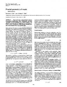
Figure 1.
The self-similarity of a snow-flake shape.
®
Figure 2.
A simple initiator and generator of a fractal shape.
mid-point along two sides of .3n equilateral triangle. The resulting line is clearly 4/3 times the length of the initiator. In Figure 2c this same generator has been applied to the curve of Figure 2b so as to produce smaller but nevertheless self-similar deviations from this line: it should be clear that there exists no reason why this same generator should not boi applied to the segments produced at each successive level until the detail become!rSo intricate that its effect is lost upon the human eye, In formal terms, Mandlebust defines fractal dimensions in terms of the number of points generated about the object/segment (N) and the "similarity ratio" (lIr) which is used to divide the initiator. Fractal dimension is then given by 0 = -log(NI/log(1/r). The line in Figure 2 has been divided into 3 parts at each stage Ir = 3). whilst 4 new parts are generated about each segment (N .. 4). Thus in our example D .. -log 4/logl 1/3) log 4/1093 which is approximately equal to 1.26. Computer Education June 1987
244
15
Figure 3(a)
Figure 3(b)
Figure 3.
The continuous space-filling 'Peano' Curve.
Figure 4(a) Figure 4.
Figure 4(b)
A fractal branching process at two levels of recursion.
Fractals and computer graphics Of course. the task of subdillision at successille scales would gradually become increasingly time-consuming and tedious. were it to be performed manually. Howeller. the graphics capabilities of ellen quite modest microcomputers are lIery amenable to this type of operation: for example. Figure 1 illustrates how the BBC micro copes with the introduction of fractal irregularity (using the same generator described abolle and illustrated in Figure 2) into a triangular initiator. The lellel at which we halle stopped this 'recursille' process has been chosen because further recursion is unlikely to reproduce effectillely in this magazine: once the generator rule has been programmed, howeller, it is feasible to allow the recursille procedure to continue until the lellel of screen resolution is reached and hence no finer-scale recursion is discernible. Figure 1 does, in fact, depict the so-called 'Koch curlle' which was first explored by Helge lion Koch in 1904, and the study of which could not be adllanced prior to the discollery of fractal geometry. Of course the Koch curlle is but a single example of the myriad of fractal lines whose dimensions lie between 1 and 2. The general rule is that as fractal dimension increases towards 2, so the fractal lines come to fill more and more space until at dimension 2 the line totally encloses space and becomes a surface. Figure 3 shows a continuous curlle which at increasing lellels of fractal recursion comes to fill space and has a dimension of 16
Computer Education
June 1987
approximately 2. Curlles with dimensions much closer to 1 ar much less intricate or 'kinky' and bear closer resemblance to straight line (dimension 1) than a surface. What, though, about fractals of dimensions greater than 2 or Ie than 1? Fractals of dimension between 2 and 3 are probably easier to understand, although they are much more complica to simulate using computer graphics. Intuitillely this is easy Ie understand if one considers a cube (of dimension 3), the bow of which is a surface (of dimension 2). Then a fractal shape wi dimension between 2 and 3 will nOI fill the entire cube bul will : more of it than the 2-dimensional surface. Simulation of fract, shapes of dimension between 2 and 3 has been used in a numt of science fiction films (notably in the 'Project Genesis' sequen of the film 'Star Trek WI to simulate computer landscapeswhi, are imaginary yet realistic. By contrast, the generation of line, with a fractal dimension of less than 1 inlloilies a recursion in which the generated lines become shorter and shorter, yet always remain of finite length. Recursion to fine lellels of resolution results in the generation of what Mandlebrot has termed 'Cantor dusts', In biology, the nautral branching prOCE of trees can be represented as a fractal of dimension approximately equal to 0.6. Figure 4a shows a branching tree dimension 0.63 at a depth of 61ellels of recursion while, in Figu 4b. extension of the branching to 131ellels of recursion genera a leaf-like 'fractal canopy'.
Whilst all of the fracta~shapes we have considered so far constitute interesting computer graphics, and whilst some of our 'pure' fractals have evident natural realism le,g, the Koch 'snowflake' in Figure 1 and the tree in Figure 4), we nevertheless might anticipate that a branch of mathematics as new and exciting as fractals might have even wider applicability in the 'real world', However, if we return to our first example of the length of a coastline, the overall fractal dimension of our snowflake 11.26) happens to be very close to that of the west coast of Britain, yet the coast clearly exhibits a much more complex pattern of irregularity than the snowflake. The key to creating fractals of greater generality lies in the introduction of a random element to our fractal recursions. Mandlebrot suggests that the basis upon which this random element might be introduced is directly analogous to the way in which hydrologist:; simulate the movement of tiny particles in a liquid. The technicalities of this technique (a model of Brownian moticn) need not detain us here, but its importance is that it leads to fractal shapes which, although not exactly self-similar as in the case of the snowflake, nevertheless do possess considerable visual realism. Implementation of the fuU technique presents a daunting task, although programming short-cuts can lead to results which exhibit no obvious deleterious effects. The generation of random fractals is thus particularly appropriate for the representation of boundaries such as coastlines, as the successive stages in the simulation of the continents of the imaginary planet reproduced in the back cover of Mandelbrot's famous (1982) book The Fractal Geometry of Nature. It is these sorts of simulation which result in some of the stunning computer graphics, particularly mountain scenes, which are being increasingly used in the movie industry. Fractal techniques in planning research The notion that fractal self-similarity need not be exact, and that it is those compound fractals which are perturbed in an inexact manner which frequently generate the most realistic images, provides the main stimulus to our use of fractals in planning' research. Just as mountain or planetscapes may exhibit random or statistical self-similarity, so cities are self-similar in an as yet undefined sense. For example the urban mosaic of residential neighbourhood types and also the juxtaposition of different urban land-uses is clearly comparable both within and between urban areas, and hence we might reasonably suppose that such patterns are fractal. In our own research in the Department of Town Planning at the University of Wales Institute of Science and Technology we have assigned fractals a central role both in the measurement of irregularity of urban boundaries and in the simulation olthe paths of urban boundaries within a given urban area (see Figure 5). This research has involved extensive use of both microcomputers and mainframe facilities. Although measurement of the structure of a line logically precedes using the measurements to simulate the form of others, for clarity of exposition, we will look at these two stages in reverse.
I-,~.~,~,'~, L______ Figure 5.
r -,.-
('~
~
"'lOBI..'
~
/'
Y = fIX" X2 , Xl) + E
(N = 3)
where Y would be coded so as to take different numerical values f~r each of our five different land-uses, X, would measure dlstanc.e from the lawn/city centre, X2 would be the number of years since the land parcel was first developed and X, would be our Index of similafity of adjacent land uses. The 'f'simply denotes that some mathematical function is being used to relate Y to the three X terms, and E is the error/residual term alluded to above. This discussion is necessarily a gross simplification of a broad sphere,of ,urban analysis which is actively taught and re~ea.rched wlt.hln our department: nevertheless. the important pn.nclple remains that such a model could be fitled to a data set uSI~g a standard technique le,g. based upon regression analysis) to YIeld parameter estimates, and the statistical 'fit' of the model cou~d ~hen be evaluated by using the sorts of confirmatory statistiCS that one encounters in an Advanced Level or an undergraduate statistics course (e.g. '\' and 'R 2 • statistics). Within planning, this sort of approach has been adopted in a wide range of applied, teaching and research contexts, both within the public and the private sector. Of course, a major role of such models in a planning context is to understand and assess how phe~om.ena ~ary across space.it is therefore a pity that many applications In the modelling tradition in planning do not move beyond indices of model fit which do not n~essariJy vary across spac:e It, R2, etc.) A means of remedying this would be to utilise computer g.raphics in order to generate large scale spatial forecasts, since an unrealistic or implausible forecast would then suggest a poor model. The difficulty nevertheless remains as how to partition the areal units in these forecasts, for maps based ~pon a coarse grid lack cartographic realism (as anyone who has Inspected a lineprinter map will testify) and hence are much more di~icult to interpret visually. The critical stumbling block within thiS approach thus resurfaces as our previous notion of visual realism. It is in this context that random fractals resume a central role for, as we have already seen fractal-based images can be created which have inherent visual plausibility. Figures 6 and 7 show how randomly generated fractal perturbations have been used to divide a 'london-like' simulation space into land parcels for four different housing types. These maps display results obtained by fitting this mOdel to a London housing data set:
YH = flDp.Atil + EH YH takes different numerical values for four different housi~g types (terraced house, purpose-built flat, convertible flat and detached/semi-detached house), Dp is the distance of the land parcel in which dwelling YHlies, and AH is the age of each housing unit YH' The terms f and EH have similar interpretations to the equivalent terms in the previous equation. Figures 6 and 7 reveal clearly different housing land use patterns: in fact, these differences reflect two different possible interpretations of our model results and we have previously described how these interpretive differences can arise (Batty and Longley, 1986). What is most important for present purposes, however, is the use of random fractual perturbations in order to generate land-use parcels lends the maps a plalJsible areal SUbdivision and makes them interpretable without the distraction of an 'un-natural' land partitioning. Figures 6 and 7 were both produced on a BBC micro computer.
A central role for fractals in urban planning research.
An end goal of much planning research lies in prodUCing successful 'mOdels' of urban areas. Such 'mOdels' are in effect a simplification of reality in which the impact of a few selected factors upon an urban form (or its functions) is assessed. This is often achieved by assuming first, that a relationship exists between a dependent variable (Y) and a convenient number IN) of independent IX" X%'••• XN ) variables, and second, that the myriad of other factors which might conceivably also enter the relationship are unimportant and can be assumed to cancel each other out in our empirical analysis. These excluded factors are accounted ~~r in an 'error'l'residual' term (E). So, for example. the probabIlity that a parcel of land is devoted to one of five alternative uses (r~sidential. commercial, industrial, parks or unused vacant land) might be 'explained' by the distance of that land parcel from the town or city centre, the length oftime since it was first developed, and some index pertaining to the land·use of adjoining land parcels (e.g. an index registering similarity of land-use). The basic form of our model for this case might therefore be:
Figure 6. London.
A probabilistic simulation ofresidential land use in
Computer Education June 1987
24G
17
Figure 7. London.
A deterministic simulation of residential land use in .
This research involving production of realistic maps using fractals in the medium of computer graphics may well provide a means of evaluating planning models. As we have seen. however. there exist innumerable possible fractal generating rules between the bounds of one and two which limit our simulation space. This then begs the question as to precisely which fractal generating rule creates the most realistic partitioning of residential land-use parcels? Clearly the best way of answering this question is to actually measure the fractal dimensions of some residenlia/land use boundaries. and then to use these results in order 10 inform the generation of our simulated lines. We have attempted this within the broader context of our research project by measuring the fractal dimension of Cardiff urban boundary in a number of time periods (similar measurements could obviously be made for London).
Figure 8.
The Cardiff urban edge in 1886. 1901. 1922 and 1949.
These boundaries are shown in Figure 8 (which was created on a mainframe computer using GIMMS software). Atleasl four different methods can be employed to derive fractal measurements. and we have elaborated details of each elsewhere (Longley and Batty, 1987). Each method involves measuring the way in which the length of a land-use boundary increases as we use increasingly fine levels of resolution to measure that boundary. In effect, we thus program a mainframe computer to tackle a very similar task to the manual measurement of the length of the British coastline using maps and atlases of different scales, just like we considered in our opening paragraphs. In fact one of our four methods actually simulates walking a pair of dividers set al diHerent widths around the Cardiff urban boundary. This is shown in Figure 9, where the computer-drawn lines illustrate the way in which dividers set at increasingly wide spacings could estimate the length of the urban edge. This Figure is a clear illustration of the way in which shorter length estimates result when larger divider widths are used and fine details are not detected. These sort of 18
Computer Education
June 1987
Figure 9. Measuring the length of the Cardiff urban edge usi,: computer-simulated 'dividers' set at a series of different width.
·.
measu rements constitute 'observations' which can then be fed into a regression analysis which then allows the fractal dimension of the boundary over a given scale range to be ascertained. An alternative boundary measurement technique involves laying an imaginary grid over the boundary and counting the number of grid cells which it passes through. Successive observations for the regression analysis are then obtained by changing the spacing of the grid cells. Eight successive Observations obtained using this procedure are shown in Figure 10. Some brief concluding comments Fractal geometry seems set to change the way in which we think about substantial areas of quite ordinary mathematics. Moreover, the enhancement of graphical capabilities on both micro and mainframe computers means that quite intricate fractal shapes can be produced using everyday computer facilities in an almost routine manner. It is in this context that fractal techniques have been incorporated into our own research and, although planning has most certainly not been the first discipline to adopt fractals to emulate its subject maner, it is in subject areas such as these that new and innovative applications of fractals are emerging. HopefuUy, these will inform more basic research and help fractal geometry to be established across the spectrum of the arts and sciences. References Batty, M. and Longley. PA (1986) The fractal simulatioll of urban structure', Environment and Planning A. 18. 1143-1179. Longley. P.A. and Batty. M. (1987) 'Measuring and simulating the structure and form of cartographic lines'. in J. Hauer, H,J.P. Timmermans and N. Wrigley lads.) Contemporary Developments in Quantitative Geography. Reidel, forthcoming. Mandlebrot, B.B. (1967). 'How long is the coast of Britain? Statistical self-similarity and fractional dimension'. Science. 155, 636-638. Mandlebrot, B.B. (1982), The Fractal Geometry of Nature, W.H. Freeman and Co., New York.
Figure 10. Measuring the length of the Cardiff urban edge by superimposing increasingly coarse computer-simulated grids.
248