this paper we develop a dynamic decomposition scheme that exploits the ... used
to solve hard problems on a grid computer to optimality in reasonable time.
18th European Symposium on Computer Aided Process Engineering – ESCAPE 18 Bertrand Braunschweig and Xavier Joulia (Editors) © 2008 Elsevier B.V./Ltd. All rights reserved.
Using Grid Computing to Solve Hard Planning and Scheduling Problems Michael C. Ferrisa, Christos T. Maraveliasb, Arul Sundaramoorthyb a
Department of Computer Sciences, University of Wisconsin - Madison, WI 53706, USA b Department of Chemical and Biological Engineering, University of Wisconsin Madison, WI 53506, USA
Abstract Production planning and scheduling problems routinely arise in process industries. In spite of extensive research work to develop efficient scheduling methods, existing approaches are inefficient in solving industrial-scale problems in reasonable time. In this paper we develop a dynamic decomposition scheme that exploits the structure of the problem and facilitates grid computing. We consider the problem of simultaneous batching and scheduling of multi-stage batch processes. The proposed method can be used to solve hard problems on a grid computer to optimality in reasonable time. Keywords: mixed-integer programming; grid computing; decomposition algorithm.
1. Introduction In a process facility, scheduling decisions are made on a daily or weekly basis. Rescheduling is common because of new order arrivals, delays in raw material deliveries, processing delays and other disruptions. Thus, an efficient solution method is required to solve the real-life problems in reasonable time frame. In this paper we consider multi-product multi-stage batch processes, where a set of orders has to be processed sequentially in multiple stages and each stage consists of parallel units (Méndez et al. 2006). In most existing methods each order is divided into a set of batches (batching problem) and then these batches are used as input to a scheduling method. This sequential approach, however, often leads to suboptimal decisions due to the trade-offs between batching and scheduling decisions. Recently, Prasad and Maravelias (2007) proposed a mixed-integer programming (MIP) model to address the simultaneous batching and scheduling of multi-stage batch processes. The proposed model can potentially lead to better solutions, but it is computationally expensive. The goal of this paper is the development of a solution method that enables us to solve real-world batching and scheduling problems simultaneously in reasonable time. The proposed method is based on a dynamic decomposition algorithm that is well suited to grid computing using the Condor resource management system.
2. Batching and Scheduling of Multi-stage Batch Processes 2.1. Problem Statement Given are a set of orders (i∈I) with demand qi and release/due time ri,/di; a set of processing units (j∈J) with minimum/maximum batch sizes bjmin/bjmax, processing time τij and processing cost cij; a set of stages (k∈K) with parallel processing units (j∈Jk; J = J1∪J2 …∪J|K|) at each stage k; a set of forbidden units FJi for order i and a set of
2
Ferris et al.
forbidden production paths (j,j′)∈FP for all orders. The goal is to determine the number and size of batches for each order (batching), the assignment of batches to processing units at each stage, and the sequencing of assigned batches in each processing unit (scheduling), so as to minimize the makespan. We assume that all orders go through all stages, unlimited storage is available for intermediates between stages, and changeover times are negligible. 2.2. MIP Formulation min max To account for the batching decisions, we have to calculate the minimum li = ⎡qi/ bˆi ⎤ max max % and maximum li = ⎡qi/ bi ⎤ possible number of batches that order i∈I can be divided max max to, where bˆi = mink∈K (maxj∈JAik bj ) is the maximum feasible batch size for order i, max max % bi = mink∈K (minj∈JAik bj ) is the largest batch size for order i that can be processed on all allowed units, and JAik = Jk\FJi is the set of units that can be used for the processing of order i in stage k. The set of potential batches for order i∈I is Li = {1, 2, …limax}. More details can be found in Prasad and Maravelias (2007). 2.2.1. Batch Selection and Assignment We introduce binary variables Zil, Xilj and continuous variable Bil to denote the selection, assignment, and size respectively of batch (i,l). Eq. (1) enforces that a batch is assigned to a processing unit at each stage if it is selected. If assigned, then the size of batch (i,l) has to be within the processing limits, as in eq. (2). Eq. (3) ensures that the demand for each order is met.
∑
X ilj = Z il
∑
b j X ilj ≤ Bil ≤
∀i , l ∈ L i , k
(1)
j∈JA ik
∑
min
j∈JAik
max
b j X ilj
∀i , l ∈ L i , k
(2)
j∈JA ik
∑B
il
≥ qi
∀i
(3)
l ∈L i
2.2.2. Batch Sequencing and Timing We introduce binary Yili’l’k that is equal to 1 if batch (i,l) precedes (i’,l’) in stage k. The sequencing and timing of batches in the same stage is accomplished via eqs. (4) and (5): X ilj + X i ' l ' j − 1 ≤ Yili ' l ' k + Yi ' l ' ilk ∀ ( i , l , i ' l ' ) ∈ IL : i ≤ i ', k , j ∈ JA ik ∩ JA i′k
Ti ' l ' k ≥ Tilk +
∑
τ i'j X i ' l ' j − M (1 − Yili ' l ' k )
∀ ( i , l , i ' l ' ) ∈ IL, k
(4) (5)
j∈JA i′k
where Tilk denotes the finish time of batch (i,l) in stage k. The timing of a batch between two consecutive stages is enforced by eq. (6), while release and due time constraints are enforced by eq. (7), where IL = {i , i ' ∈ I , l ∈ L i , l ' ∈ L i′ : ( i ≠ i ' ) ∨ ( ( i = i ' ) ∧ ( l ≠ l ' ) )} is the set of all combinations of batches that can be sequenced on a unit:
Ti ,l , k ≥ Tilk −1 +
∑τ
ij
X ilj
∀i , l ∈ Li , k
(6)
j∈JAik
ri Z il +
∑∑ k ' ≤ k j∈JA ik ′
τ ij X ilj ≤ Tilk ≤ d i Z il −
∑∑ k ' > k j ∈JA ik ′
τ ij X ilj
∀i , l ∈ Li , k
(7)
Using Grid Computing to Solve Hard Planning and Scheduling Problems
3
2.2.3. Additional Constraints We introduce eq. (8) to exclude infeasible assignments. Eq. (9) takes care of forbidden paths, while eqs. (10) and (11) are used to avoid symmetric solutions:
∑ ∑τ
ij
X ijl ≤ MS − min i∈IA j
i∈IA j l ∈Li
X ilj + X ilj ' ≤ Z il
Z il +1 ≤ Z i ,l Bil +1 ≤ Bi , l
{∑ k '> k
} {
}
min( τ ij' ) − min ri + ∑ min( τ ij ' ) j '∈J k ′
i∈IA j
k '< k
j '∈J k ′
∀k , j ∈ J k
(8)
∀i ∈ I , l ∈ L i , ( j , j ') ∈ FP
(9)
∀i , l ∈ L i
(10)
∀i ∈ I , l ∈ L i
(11)
Integrality and non-negativity constraints are expressed by eq. (12). Z il , X ilj , Yili ' l ' k ∈ {0,1}
Bil , Tilk ≥ 0
(12)
where IAj=I\FIj is the set of orders that can be assigned to unit j. min
We also fix all variables for l∉Li to zero. Finally, we fix binaries Zil to 1 for l ≤ li . 2.2.4. Objective The objective is to minimize the makespan MS, which is greater than the finish time of all batches at the last stage. min MS (13)
MS ≥ Til |K |
∀i ∈ I, l ∈ Li
(14)
The MIP model P consists of eqs. (1) – (14). Note that the model has an inherent hierarchy of decisions: a selected batch is assigned to a single unit in each stage via eq. (1), and a sequencing binary is activated if two batches are assigned to the same unit via eq. (4).
3. Grid Computing Grid Computing utilizes a pool of computers as a common resource in an opportunistic manner. It does not require dedicated computers, but it simply uses distributively owned computational resources and facilitates better utilization of CPU power. We use the Condor resource manager (Epema et al., 1996) that manages a large collection of Linux-based machines at University of Wisconsin Madison. However, Condor can be used on other machine architectures and operating systems (Windows, Solaris) as well. We implement the proposed solution approach for this problem using GAMS/Grid options (Bussieck et al., 2007). We adopt the master-worker paradigm as a model of computation, where model P is decomposed into a number of subproblems (tasks). The master processor generates and spawns all the subproblems, and also collects the results of each subproblem (see Figure 1). A separate task directory is created for each subproblem by the master processor. Condor submits the subproblems to worker processors for execution. Condor does not require a shared file system between the master and the workers. Instead, it simply ships the subproblem directory to a “sandbox” on the worker machine, which in turn executes the subproblem within the sandbox. Once the subproblem is completed, a file “finished” is created in the subproblem directory of the master processor along with the requisite solution files. The
4
Ferris et al.
appearance of the “finished” file and the solution loading process are carried out in GAMS using the “handlecollect” primitive. Communication between the master and worker processors is implemented via the Condor_chirp utility. When a new incumbent is found, the utility updates the master processor by creating a “trigger file” in the task directory. Further, it uses the current best incumbent from the master processor to prune/continue the subproblem in other worker processors. Examples of the GAMS syntax used for grid submission, and the methods that deal with different grid engines are discussed in Bussieck et al. (2007). “handlecollect” repeatedly checks for “finished” files Separate directory for each subproblem
“finished” file upon completion of subproblem
Master …
Co
“trigger” file is created if new incumbent is found
or nd
Worker 1
Worker 2
Sandbox
Sandbox
…
Worker N Sandbox
condor_chirp utility Fetch: copies trigger file Remove: removes trigger file after copying Put: places new incumbent in master directory
Figure 1. Architecture for Optimization on the GAMS/Grid using Master-worker Paradigm.
4. Dynamic Decomposition Algorithm 4.1. Strong Branching Our goal is to dynamically decompose original model P into smaller subproblems that can be solved using Grid computing. Unlike static decomposition, where subproblems are generated a priori, dynamic decomposition generates subproblems over the time as and when required. We first used strong branching with the goal of generating subproblems that are easier than problem P. Based on the size of the grid engine, problem P is partitioned using strong branching into a number of subproblems (open nodes), which are submitted to worker processors. Subproblems that remain unsolved after a resource limit, are re-partitioned using strong branching. The process is repeated dynamically as necessary until, in principle, all subproblems are easy to solve (Figure 2a). Nevertheless, our preliminary results indicated that strong branching does not always lead to easier subproblems. Specifically, some of the open nodes correspond to problems that are almost as hard as the original problem P. This motivated us to develop a domain-specific decomposition method. 4.2. Proposed Decomposition Our solution method exploits the inherent structure of the problem to sequentially decompose original model P into subproblems of different levels of complexity (Figure 2b). Subproblems are generated by fixing batch selection Zil and batch-unit assignment Xilj binary variables. 4.2.1. Fixing Selection of Batches The 1st-level subproblems are generated by fixing the number of batches for each order i∈I. If li denotes the number of batches that are fixed for order i∈I, then each subproblem is generated by setting li = limin = limax, ∀i∈I in eqs. (1) – (14) of model P. Note that we consider all possible combinations of li between limin and limax for a given set of orders.
Using Grid Computing to Solve Hard Planning and Scheduling Problems
5
4.2.2. Fixing Batch-unit Assignments If any of these 1st-level subproblems remains unsolved within a resource limit (typically 1 hr), then it is decomposed into a set of 2nd-level subproblems by fixing batch-unit assignment decisions at one stage kF (typically the bottleneck stage). If any of these 2ndlevel subproblems remains unsolved, then it is further decomposed into 3rd-level subproblems by fixing batch-unit assignment decisions at another stage. This process can be repeated multiple times, or it can be followed by the dynamic decomposition based on strong branching (section 4.1). P
Master
P 1st-level subproblems by fixing Zil Worker 2
Worker 1 Promising Worker 3
Non-promising
Worker 4
Promising Non-promising
a) Strong-branching-based decomposition
2nd-level subproblems by fixing Xilj in one stage 3rd-level subproblems by fixing Xilj in another stage
b) Domain-specific decomposition
Figure 2. Dynamic decomposition based on a) strong branching and b) problem structure (grey nodes denote hard subproblems that need to be decomposed further).
The number of different batch-unit assignments is very large even for medium size problems. Some of these assignments lead to promising subproblems(i.e. subproblems that are likely to yield a good solution), while others lead to non-promising ones. Although non-promising subproblems are easy to prune, the resources required for their generation, submission and solution are substantial. To avoid generating a large number of such tasks, we identify a subset of assignments that are likely to lead to good solutions and solve each one of them separately, while subsets of non-promising assignments are lumped into larger subproblems that are easier to prune. To this end, we use the idea of balanced batch-unit assignments: a min makespan schedule is likely to have the load in the bottleneck stage distributed almost equally among units. Thus, subproblems that correspond to balanced assignments are generated by fixing all variables Xilj at stage kF: X ilj = 1,
∀j ∈ J k F , (i , l ) ∈ D j
(15)
where set Dj is the set of batches that are assigned to unit j in the current subproblem. Non-promising subproblems are generated by adding either of the following constraints for each unit in stage kF:
∑X
≤ NJ
MIN
ilj
−1
(16)
≥ NJ
MAX
ilj
+1
(17)
i ,l
∑X i ,l
where NJMIN (NJMAX) is an estimate of the number of batches that if assigned to a single unit makes it highly (lightly) loaded. In this paper we use NJMIN = ⎣0.9M/|J(kF)|⎦ and
6
Ferris et al.
NJMAX = ⎡1.1M/|J(kF)|⎤, where M is the total number of batches in the current subproblem and |J(kF)| is the number of units in stage kF. Note that promising subproblems have all batch-unit variables fixed in stage kF from eqs. (1) and (15) but are hard to solve due to their poor lower bounds. On the other hand, non-promising subproblems are less tightly constrained by eq. (16) or (17) but are pruned easily because they encompass many but unbalanced assignments, thus have high lower bounds. Finally, we developed a pre-processing procedure in order to identify infeasible batchunit assignments. First, we remove subproblems with the forbidden batch-unit assignments. Then, we check the capacities of units to ensure that the demands of orders are met. Finally, when variables Xilj are fixed in more than one stage, we remove the subproblems with forbidden paths. The proposed procedure improves the performance of our algorithm by screening infeasible subproblems a priori, thus reducing the time required to generate, spawn and solve a number of subproblems.
5. Results We present results for a process that consists of three stages with two units per stage and 10 orders. We consider two instances of this problem: instance 1 results in a problem with 10-11 batches, while instance 2 with 12-15 batches. The problem data are available from the authors. We analyzed the effect of both the automatic decomposition scheme based solely on strong branching (scheme 1) and the domain-specific decomposition (scheme 2). Instance 1 was solved to optimality in almost 2 hr of wall clock time and 2,905,742 nodes using scheme 1. In scheme 2, we carried out the 1st-level domain-specific decomposition and then followed with decomposition based on strong branching. Instance 1 was solved in only 7.5 min of wall clock time and 9,601 nodes. For instance 2, scheme 1 failed to solve the problem due to the generation of innumerable subproblems. On the other hand, scheme 2 solved the problem to optimality in 9 hr of wall clock time exploring 222,065,793 nodes. In this case, we carried out the 1st, 2nd and 3rd level domain-specific decompositions followed by strong branching. In this paper we proposed a solution method to solve the problem of simultaneous batching and scheduling in multi-stage multi-product processes. Our method uses GAMS/Grid options and grid computation facilitated by the Condor management system. It couples problem-specific knowledge with strong branching to dynamically decompose hard problems into a set of subproblems. Our computational studies showed that the proposed method can be used to solve hard problems to optimality with reasonable time. Finally, we note that the proposed methodology can be applied to a wide range of production planning and scheduling problems.
References Bussieck, M., Ferris, M. C., Meeraus, A., 2007. Grid Enabled Optimization with GAMS. Technical Report, Computer Sciences Department, University of Wisconsin. Epema, D. H. J., Linvy, M., van Dantzig, R., Evers, X., Pruyne, J. 1996. A Worldwide Flock of Condors: Load Sharing among Workstation Clusters. Future Generation Computer Systems 12, 53-65. Méndez, C.A., Cerda, J., Grossmann, I.E., Harjunkoski, I., Fahl, M., 2006. State-of-the-art Review of Optimization Methods for Short-term Scheduling of Batch Processes. Comput. Chem. Eng. 30, 913-946. Prasad, P., Maravelias, C.T., 2008. Batch Selection, Assignment and Sequencing Multi-stage Multi-product Processes. Comput. Chem. Eng., (doi:10.1016/j.compchemeng.2007.06.012).