Appears in Proceedings of the 38th International Conference on Dependable Systems and Networks (DSN), June 2008.
Using Likely Program Invariants to Detect Hardware Errors
∗
Swarup Kumar Sahoo, Man-Lap Li, Pradeep Ramachandran, Sarita V.Adve, Vikram S. Adve, Yuanyuan Zhou Department of Computer Science University of Illinois at Urbana-Champaign
[email protected]
lutions such as variations on redundant multithreading improve on this, but still incur significant overheads [27]. Recently, researchers have investigated using softwarevisible symptoms to detect hardware errors [5, 9, 19, 24, 25, 26, 30, 32]. While much of that work focuses on transient or intermittent faults that last a few cycles (e.g., 4 cycles or less), we have explored using these symptoms to detect permanent faults in hardware [9]. Using software-level symptoms to detect permanent faults in hardware has several benefits over traditional hardwarelevel solutions. First, using software-level symptoms deals with only those errors that actually affect software correctness. The rest of the faults are safely ignored, potentially reducing the incurred overhead due to detection and recovery. Second, the reliability targets for the system under consideration dictates the overheads that the system allows to achieve those targets. Using software-level symptoms for detection facilitates exploring these trade-offs in reliability and overhead seamlessly as they are highly customizable. We proposed a system design called SWAT, a firmwarelevel low-overhead reliability solution that could potentially handle multiple sources of hardware failures [9] using software symptoms such as fatal hardware traps, software hangs, abnormal application execution, and high OS activity. Implementing these detectors in a thin firmware layer would present significantly lower hardware cost than using traditional circuit-level hardware detectors. These detectors help identify over 95% of hardware faults in many structures. Additionally, 86% of these detections can be recovered using hardware checkpointing schemes, while all these detected faults are software recoverable [9]. Nevertheless, using these simple symptoms as detectors results in an SDC rate of 0.8% for permanent hardware faults in the current SWAT system, which may not be acceptable for most systems. This motivates the use of more sophisticated detectors to further reduce this SDC rate and increase detection coverage. In addition, using more sophisticated detectors has the potential of reducing the detection latency of the detected faults, making more faults amenable to hardware recovery. Recovery through hardware checkpointing techniques, which can treat detection latencies upto 100K
Abstract In the near future, hardware is expected to become increasingly vulnerable to faults due to continuously decreasing feature size. Software-level symptoms have previously been used to detect permanent hardware faults. However, they can not detect a small fraction of faults, which may lead to Silent Data Corruptions(SDCs). In this paper, we present a system that uses invariants to improve the coverage and latency of existing detection techniques for permanent faults. The basic idea is to use training inputs to create likely invariants based on value ranges of selected program variables and then use them to identify faults at runtime. Likely invariants, however, can have false positives which makes them challenging to use for permanent faults. We use our on-line diagnosis framework for detecting false positives at runtime and limit the number of false positives to keep the associated overhead minimal. Experimental results using microarchitecture level fault injections in full-system simulation show 28.6% reduction in the number of undetected faults and 74.2% reduction in the number of SDCs over existing techniques, with reasonable overhead for checking code.
1. Introduction As CMOS feature sizes continue to decrease, hardware reliability is emerging as a major bottleneck to reap the benefits of increasing transistor density in microprocessor design. Chips in the field are expected to see increasing failure rates due to permanent, intermittent, and transient faults, including wear-out, design defects, soft errors, and others [2]. The traditional approach in microprocessor design of presenting an illusion of a failure-free hardware device to software will become prohibitively expensive for commodity systems. Traditional solutions such as dual modular redundancy for tolerating hardware errors incur very high overheads in performance, area and power. Recent hardware so∗ This
work is supported in part by the Gigascale Systems Research Center (funded under FCRP, an SRC program), the National Science Foundation under Grants NSF CCF 05-41383, CNS 07-20743, and NGS 04-06351, an OpenSPARC Center of Excellence at the University of Illinois at UrbanaChampaign supported by Sun Microsystems, and an equipment donation from AMD.
1
cycles [28], are more attractive than those that use software checkpointing techniques for recovery as it facilitates seamless recovery of both the application and the OS in the event of a fault with much lesser overhead. In this work, we extend the set of symptom-level detectors in SWAT to include program-level invariants that are derived from program properties observed during program execution. We use “likely program invariants” which have been shown to be a powerful approach in detecting software bugs [4, 6]. We derive likely program invariants by monitoring the execution of a program for different inputs and identifying program properties that hold on all such executions. 1 A major drawback with using likely invariants for error detection is that they may lead to false positives: some of the inferred program invariants may be violated for an input as the program behavior on that input is different compared with the training inputs used to extract invariants. Hence, likely program invariants have been proposed and used primarily for analysis purposes such as program evolution [4], program understanding [7], and detecting and diagnosing software bugs [4, 6, 12, 33, 13]. The only exceptions have been for detecting transient hardware faults, where a false positive can be identified quickly and cheaply [22, 24, 3]. In this paper, we propose and evaluate a hardwareassisted methodology to use likely invariants for detecting permanent (or intermittent) hardware errors safely. The SWAT system has a hardware-assisted diagnosis framework and we adapt it to detect false positives at runtime. We also limit the number of false positives in a novel way to keep the associated overhead due to false positive detection low. Using the principles discussed above, we designed the iSWAT framework for invariant detection and enforcement, and we implemented it as an extension of the SWAT system [9]. The contributions of this work are: • We demonstrate a new hardware-supported strategy for
using unsound program invariants for detecting permanent hardware errors. We believe this is the first work to use unsound invariants for such errors.
• We show that likely invariants can be extracted efficiently
in software for realistic programs, unlike previous work which used only toy benchmark programs [22]. Furthermore, because of our tolerance for false positives, we only need 12 inputs for extracting our invariants while others have used hundreds of inputs [4, 22].
• We provide a realistic and comprehensive evaluation
with full-system simulation by injecting faults into different micro-architectural structures. Such faults present more realistic fault scenarios than the previously studied application-level fault injections.
1 With
simple compiler support, this “training” phase can be performed transparently during debugging runs for any program, and could even be extended into production runs with more sophisticated tools [11].
• The most important outcome from our experiments is that
our technique reduces SDCs by 74.2%: fewer than 0.2% of all fault injections are now SDCs.
In more detail, our experimental results show that the number of undetected faults in iSWAT decreases by nearly 28.6% compared with the base SWAT System. The number of SDCs reduces from 31 to 8 (i.e., 74.2% reduction). The number of detections that are hardware recoverable (with latency less than 100K instructions) improves slightly by 2%. The mean overhead due to invariant checking code is low - 14% on an UltraSparcIIIi machine and only 5% on an AMD Athlon machine. Moreover, this work is just a first step using one simple style of invariants. These results show that using likely invariants is a promising way to improve overall reliability, at a low cost. The rest of this paper is organized as follows. Section 2 provides a brief overview of likely invariants. In Section 3, we describe the iSWAT System in detail, explaining how we exploit the diagnosis module to detect false positives caused by the invariants. Section 4 discusses the evaluation methodology, the results of which are discussed and analyzed in Section 5. Related work is discussed in Section 6. Section 7 draws conclusions and implications from our experience with the iSWAT framework and discusses future work.
2. Invariant-Based Error Detection In this section, we provide some background on likely program invariants and then discuss the particular type of likely invariants we use to detect permanent faults. 2.1 Likely Program Invariants A program invariant at a particular program point P is a property that is guaranteed to hold at P on all executions of the program. Static analysis is the most common method to extract such sound invariants. A combination of offline invariant extraction pass and static analysis, or theorem proving techniques, has also been suggested to extract sound invariants [20]. However, current techniques are not scalable enough to generate sound invariants for real programs [20]. Also, they can not identify algorithm-specific properties that are not explicit in the code (e.g. some inputs are always positive). Likely Program Invariants are properties involving program values that hold on many executions on all observed inputs and are expected to hold on other inputs. However, they are unsound invariants which may not hold on some inputs. Extracting likely program invariants is easier than extracting sound invariants as we do not need expensive static analysis methods to prove program properties and can identify algorithm specific properties. The extraction can be done either online or offline. In online version, invariants are extracted and used during program execution in the production runs. Online extraction can present unacceptable overheads
to program execution, and may in fact be infeasible without hardware support. The offline version, on the other hand, extracts invariants in a separate pass during program testing or debugging, and these generated invariants can be used later during the production runs. During the testing phases of software development, the extra overhead of invariants extraction can be tolerated. This makes offline invariant extraction a powerful method, allowing the use of more complex invariant mining techniques than would be feasible with online methods. With compiler support, this “training” phase can be done transparently at development time. We can broadly classify likely program invariants into three categories. Value-based invariants specify properties involving only program values, and can be used for a variety of tasks including software bug detection, program understanding and program refactoring etc [4, 11, 7, 12, 6]. Control-flow-based invariants specify properties of the control flow of the program, and have been used previously to detect control-flow errors due to transient faults [30, 29, 5]. PC-based invariants specify program properties involving program counter values, and have been proposed for detecting memory errors in programs during debugging [33]. 2.2 Range-Based Invariants One of our main goals in exploring the use of invariants to detect permanent faults is to improve the coverage of detection and reduce the number of SDCs. Since SDCs are typically caused by erroneous values written to output, we explore the use of value-based invariants to detect permanent faults. The other two class of invariants can detect controlflow or memory errors, which generally result in anomalous software behavior that can be detected by the other detectors in SWAT. For example, erroneous control-flow typically results in a crash which can be caught by the FatalTrap symptom in SWAT [9]. In contrast, we expect value-based invariants to capture deviations of values that do not result in any significant change of program behavior to cause an application or OS crash, but may still result in incorrect output. As a first step towards using likely program invariants for permanent hardware faults, we use a particular form of value-based invariants known as range-based invariants. A range-based invariant on a program variable x will be of the form [MIN, MAX], where MIN and MAX are constants inferred from offline training such that M IN ≤ x ≤ M AX is true for all the training runs. These range-based invariants are suitable for error detection for various reasons. These types of invariants can be easily and efficiently generated by monitoring program values. They are also composable – the invariants can be generated for each training input separately and can then be combined together to generate invariants for the complete training set. These invariants are also much easier to enforce within the checking code compared to other forms of invariants as they are simple and involve a single data value. In the ongoing future work, we are exploring a broader class of invariants.
3. The iSWAT Detection Framework We implement the above described range-based invariants as an extension to the existing SWAT System [9] to build the iSWAT system that uses likely program invariants as an additional software-level symptom to detect hardware faults. 3.1 Overview of SWAT System The SWAT system uses low-overhead software-level symptoms to detect the presence of an underlying hardware faults, and exploits a firmware-assisted diagnosis and recovery module to recover the system from multiple sources of faults [9]. While this paper targets permanent hardware faults, our methods, similar to SWAT, also extend readily to detect transient faults. SWAT assumes a multi-core architecture under a single fault model where a fault-free core is always available. The system also assumes support for a checkpoint/rollback/replay mechanism and a firmware layer that lies between the processor and the OS to monitor and control such mechanisms. Detection: SWAT uses four low-cost symptom-based detection mechanisms that require little new hardware or software support. These mechanisms look for anomalous software execution as symptoms of possible hardware faults. We briefly describe them below; the details can be found in [9]. 1. FatalTrap: Fatal hardware traps are those traps (caused by either the application or the OS) that do not occur during fault-free execution. In Solaris, some of the fatal traps are RED (Recover Error and Debug) State trap, Data Access Exception trap etc. 2. Abort-App: These indicate instances of a segmentation fault or illegal operation, when the OS terminates the application with a signal. In such cases, the OS informs the detection framework that the application performed an illegal operation, leading to a detectable symptom. 3. Hangs: Application and OS hangs are other common symptoms of hardware faults [19]. SWAT uses a low hardware-overhead heuristic hang detector, based on (offline) application profiling to detect hangs with high fidelity. 4. High OS activity: In normal executions, on a typical invocation of the OS, control returns to the application after a few tens of OS instructions, except cases such as timer interrupt or I/O system calls. As a symptom of abnormal behavior, SWAT looks for instances of abnormally high contiguous OS instructions to indicate the presence of an underlying fault. Diagnosis: After the fault detection, the diagnosis framework is invoked to distinguish the source of the fault as a software fault, or a transient fault, or a permanent fault. The diagnosis component rolls back to the last checkpoint and replays the execution on the original core. If the symptom
does not recur, it infers a transient fault and continues execution. However, if the symptom recurs, it re-executes on another core (assumed to be fault-free) to distinguish software faults (in which case the symptom would most likely reoccur on the fault-free core) from permanent hardware faults (in which case the symptom would not occur). We may need to do the replay multiple times on the two cores to distinguish not-deterministic software errors. In the case of a permanent fault, the diagnosis module also does microarchitecture level diagnosis to identify the faulty microarchitectural structure [10]. Recovery and Repair: For recovery, SWAT assumes some form of checkpoint/restart mechanism that periodically checkpoints the state of the system. Depending upon the requirements, appropriate hardware checkpointing or software checkpointing mechanisms, or a combination of both, can be used to recover the system after detection. SafetyNet [28] and Revive [18, 23] show reasonably low overhead for hardware checkpoint/replay. In the event of a permanent hardware fault, the component that is diagnosed as faulty can be reconfigured or disabled. 3.2 The iSWAT system The iSWAT system extends the above described SWAT system to include the violation of likely program invariants as possible symptoms that indicate the presence of a hardware fault. These invariants are derived from “training” runs of the application and the invariant checking code is embedded into the application. iSWAT exploits the diagnosis and recovery module of the SWAT system to detect and disable false-positive invariants at run-time. 3.2.1 Generating Invariants and Invariant Checks The iSWAT system leverages support from the compiler for two distinct components: invariant generation and invariant insertion. Both of these use the LLVM compiler infrastructure [8]. Invariant Generation: We use compile-time instrumentation to monitor program values during training runs in order to generate likely program invariants. We can monitor many different types of values, including load, store, return and intermediate result values. For this work, we decided to monitor only the store values as checking values stored to memory has the most potential to catch faults, as all necessary computations eventually pass their results to stores. Also, monitoring only the stores helps us keep the overhead of detection low. We monitor stored values of all integer types (both signed and unsigned) of size 2, 4, and 8 bytes as well as single and double precision floating point types. We do not monitor integer stores of size 1 byte (character data types), as they represent only a small range of values and hence may be ineffective to detect faults.
We do the code generation for invariant generation in two steps. In the first step, we use LLVM-1.9 with llvm-gcc-3.4 to generate the LLVM bytecode and run an instrumentation pass to insert calls to monitor the store values. Then we generate a C program from the LLVM bytecode file through the LLVM C back end. Finally, we generate SPARC native code through the Sun cc compiler. We use the generated program to create the invariants for each input separately, which we then combine to form the final invariants in another offline pass. Invariant Insertion: The invariants generated by the offline pass then need to be inserted into the code to check the values being stored. For this, we take the invariant ranges from the generation phase and then insert calls to the invariant checking code at the LLVM byte-code level through another compile-time instrumentation pass. Then, as in the invariant generation phase, we generate a C program from LLVM bytecode through LLVM C back end and finally, use Sun cc compiler to generate native code. 3.2.2 Handling False-Positive Invariants False positives present a major short-coming for likely program invariants as detecting them may incur high overheads in the presence of permanent faults. For transient hardware faults, relatively low-cost techniques such as pipeline flush can help to tolerate false positives [24]. If the fault occurs again after pipeline flush, the invariants will be updated and this is done cheaply using hardware support. In contrast, for a framework like iSWAT System that supports permanent fault detection, more expensive rollback and replay on the same and a fault-free core is needed to detect false positives. Too many false positive detections may thus lead to exorbitant overheads. While training with too many inputs can potentially make false positives rare, the ranges may become too broad rendering the invariants ineffective for error detection. In our framework, we propose to train with a set of inputs such that the false positive rate is sufficiently low. In general, the number of false positives can be used to guide how many inputs to use for training. iSWAT leverage the existing diagnosis framework in the SWAT system [10] to detect the remaining false positives at run-time. In the event of an invariant violation, we follow the full rollback and replay on the same and fault-free core. If the violation occurs even on fault-free core, then it is a false positive invariant(or a software bug). Since too many rollback/replays due to false positives can cause large overheads, we disable the static invariants once it results in a false positive during dynamic execution (Online updation of invariants will add too much overhead for our software-only technique). In this way, if the total number of static invariants is I, the maximum number of rollbacks possible will also be I, limiting the overhead incurred due to false positives. Currently, the disable operation is done inside the invariant
i f ( ( v a l u e < min ) o r ( v a l u e > i f ( FalsePosArray [ InvId ] ! = i f ( detectFalsePos ( InvId ) FalsePosArray [ InvId ] = } }
max ) ) { / / I n v a r i a n t t r u e ) { / / Not f a l s e = = t r u e ) / / Perform true ; / / Disable the
violated positive diagnosis invariant
Figure 1. Invariant checking code template checking code and does not need any extra hardware support. We maintain a table with one entry for each invariant indexed by the invariant id to identify false positive invariants. In the invariant checking code, the table entry is marked to disable the false positive invariants from all later executions, if the invariant is detected as a false positive. Figure 1 shows a template of the actual invariant checking code. The overhead caused by false positives in an invariantbased approach depends on the number of rollbacks, which in turn depends on the number of static false positive invariants. The false positive results, presented in Section 5, indicate that the overhead for our set of applications is negligible compared to their runtimes.
4. Methodology 4.1 Simulation Environment For the fault injection experiments, we used a full system simulation environment comprising the Virtutech Simics full system simulator [31] with the Wisconsin GEMS timing models for the microarchitecutre and the memory [14] as in [9]. These simulators provide cycle-acurate microarchitecture level timing simulation of a real workloads running on a real operating system (full Solaris-9 on the SPARC V9 ISA) on a modern out-of-order superscalar processor and memory hierarchy (Table 1). We exploit the timing-first approach of the GEMS+Simics infrastructure [15] to inject microarchitecture-level faults. In such an approach, GEMS and Simics compare their full architectural states after each instruction and in case of a mismatch GEMS state is updated with Simics state. This checking mechanism was leveraged for our fault injection. The faults are injected into GEMS’s micro-architectural state and the fault is allowed to propagate. After a mismatch between Simics and GEMS, if the mismatch is found to be because of the fault, we copy the faulty architectural state from GEMS to Simics, to make sure Simics follows the same corrupted execution path as GEMS. Otherwise, the GEMS state is updated as usual. When we find the architectural state is corrupted, we say that the fault has been activated. 4.2 Fault Model In the current work, we focus on permanent or hard faults. The well established stuck-at-0 and stuck-at-1 fault models as well as the dominant-0 and dominant-1 bridging fault models are used for modeling permanent hardware faults in this paper. The stuck-at fault models model a fault in a single bit and the bridging fault model models faults that affect adjacent bits. The dominant-0 bridging fault acts like
Base Processor Parameters Frequency 2.0GHz Fetch/decode/execute/retire rate 4 per cycle Functional units 2 Int add/mult, 1 Int div 2 Load, 2 Store, 1 Branch 2 FP add, 1 FP mult, 1 FP div/Sqrt Integer FU latencies 1 add, 4 multiply, 24 divide FP FU latencies 4 default, 7 multiply, 12 divide Reorder buffer size 128 Register file size 256 integer, 256 FP Unified Load-Store Queue Size 64 entries Base Memory Hierarchy Parameters Data L1/Instruction L1 16KB each L1 hit latency 1 cycle L2 (Unified) 1MB L2 hit/miss latency 6/80 cycles
Table 1. Parameters of the simulated processor Microarchitecture structure Instruction decoder Integer ALU Register bus Physical integer register file Reorder buffer (ROB) Register alias table (RAT) Address gen unit (AGEN) FP ALU
Fault location Input latch of one of the decoders Output latch of one of the integer ALUs Bus on the write port to the register file A physical reg in the integer register file Source/dest reg num of instr in ROB entry Logical → phys map of a logical register Virtual address generated by the unit Output latch of one of the FP ALUs
Table 2. Microarchitectural structures in which faults are injected.
a logical-AND operation between the adjacent bits that are marked faulty, whereas the dominant-1 bridging faults act like a logical-OR operation. The microarchitectural structures and locations where the faults are injected are listed in Table 2. For each structure, a fault is injected in each of 40 random points in each application (after the initialization phase in each application is over). For each application injection point, we perform an injection for each of the 4 fault models (two stuck-at and two bridging faults). The injections are performed on a randomly chosen bit in the given structure. This gives a total of 800 fault injection simulation runs per microarchitectural structure (5 applications × 40 points per application × 4 fault models) and 6,400 total injections across all 8 structures. After a fault is injected, we run the simulation for 10 million instructions. Note that the fault is maintained for the rest of the 10M instruction window. For the small number of runs where an activated fault is not detected within this window, we use functional (full-system) simulation to run the application to competition (as detailed simulation is too slow to run to completion) for evaluating masking due to the application, and SDCs. The functional simulation does not inject any faults beyond the first 10M instructions, resulting in the fault acting like an intermittent fault that is active only in the 10 million instruction window. We believe that 10M instructions is long enough that the simulation reflects the behavior of permanent faults.
80%
We show the effectiveness of our invariant-based approach by evaluating invariants in conjunction with the four lowcost detection mechanisms built into the base SWAT system. This is more realistic than studying only detections by invariants as the other techniques are lower overhead (and need very little hardware/software support) and will show the impact of the new technique in any realistic system.
70%
False Positives Rate
4.3 Fault Detection Techniques Used
mcf gzip bzip2 parser art
60% 50% 40% 30% 20% 10% 0% 2
4.4 Fault Metrics When the fault causes a corruption in the architectural state of the processor, we say it is activated. If the fault is never activated, we say the fault is architecturally masked. An activated fault which is undetected, but does not cause any corruption in the output produced by the application is said to be application masked. We used five metrics to evaluate the impact of the new detection technique: 1. Coverage: The percentage of non-masked faults that are detected in the 10M instruction window. We refer the percentage of undetected faults as unknown-fraction. 2. Latency: The total number of instructions retired from the first architecture state corruption (of either OS or application) until the fault is detected by one of the above techniques. 3. SDCs: The number of SDCs which result in corrupting the output of the application. 4. False positives: The total number of false positive invariants. 5. Overhead: The overhead of the invariant checking code as a percentage of original execution time, measured in fault-free run. 4.5 Applications For the experiments, we used five SpecCPU 2000 benchmarks – four SpecInt benchmarks (gzip, bzip2, mcf, parser) and one SpecFP benchmark (art). For most of the other SPEC benchmarks, we could not collect sufficient training inputs, while we could not compile and run the others in our simluator. Previous work on invariants uses toy Siemens benchmarks because many inputs are available for these benchmarks [4, 22]. We use more realistic applications which makes it much harder for us to obtain valid inputs for experiments. Nevertheless, obtaining inputs will not be a problem in practice as developers test their programs on many inputs during the testing phase. Invariant generation and insertion can be easily done during testing through a compiletime pass. The “test” and “train” input sets formed part of our training set. Different techniques were used to generate more inputs depending on the benchmarks. For three benchmarks (gzip, bzip2 and parser), we collected random inputs
4
8
12
Number of Training Inputs
Figure 2. Variation of False positives rate with different number of training inputs. The rate is