Using LISREL and PLS to Measure Customer Satisfaction - CiteSeerX

Using LISREL and PLS to Measure Customer Satisfaction

Lynd D. Bacon, Ph.D. Lynd Bacon & Associates, Ltd. [email protected] http://www.lba.com Seventh Annual Sawtooth Software Conference La Jolla CA Feb. 2-5, 1999

Using LISREL and PLS to Measure Customer Satisfaction Lynd D. Bacon, Ph.D. There’s a consensus that customer satisfaction is important. There have been numerous books, articles, and conferences devoted to it and its determinants. Firms have invested huge amounts in collecting satisfaction data, analyzing them, and reporting on the results. Satisfaction has been argued to be a critical component of brand equity (e.g. Aaker, 1991). Firms and managers perceive it to be related to customer retention, which is related to profitability. Governments have funded national studies to monitor it. Although other constructs have been proposed to be more important correlates of loyalty (e.g. customer value, see Gale, 1994), it is definitely the case that customer satisfaction is a central construct in the relationship between firms and customers. Researchers and managers have used a variety of definitions for customer satisfaction. Most refer to a psychological process involving prior knowledge, beliefs, or expectations; perceived performance; and the evaluation of this information, or an affective response to it. Oliver (1997, p. 13) provides the following general definition:

Satisfaction is the consumer’s fulfillment response. It is a judgment that a product or service feature, or the product or service itself, provided (or is providing) a pleasurable level of consumption-related fulfillment, including levels of under- or over overfulfillment. It’s important to note that the fulfillment response Oliver refers to is internal to the customer. Satisfaction is unobservable Unlike physical quantities like temperature or weight, the extent of a customer’s satisfaction must be inferred. It is assessed by what Torgerson (1958) called measurement by fiat. Since we can’t measure it directly, we instead measure other variables that are observable. These are sometimes called indicator, or manifest, variables. Based on a priori grounds, or perhaps on more sophisticated procedures, we ascribe meaning to what we observe based on the presumed relationship between satisfaction and our indicator variables. Unobserved, or latent, variables are very common in marketing research. They include real income, socioeconomic status, perceived quality, utility, brand attitude, purchase intention, and loyalty. To measure them we rely on observable indicators that are (hopefully) correlated with them.

1998 Sawtooth Software Conference ©1999 LBA: Lynd Bacon & Associates, Ltd. All Rights Reserved -1-

It’s important not to treat indicators and the latent variables that may underlie them as being the same thing. We should observe the Chinese proverb (Bagozzi, 1994a): "Do not confuse the finger pointing at the moon with the moon." Now it’s probably unlikely that many managers or researchers truly believe that the numeric responses elicited by satisfaction measurement scales really are satisfaction per se. Yet the practice of reporting and modeling the observed responses while ignoring any errors in measurement that may be present, can mislead. One reason is that estimates of the correlation between satisfaction and other variables will be biased. Some form of correlational analysis is often used to do what’s called "key driver analysis" (Oliver, 1997) or "revealed preference analysis" (Hauser, 1991) in satisfaction research, so the effects of measurement error have practical implications. Effects of unreliability The reliability of a measure is the extent to which it provides consistent results from one application to the next, or the degree to which it is free of random error (Vogt, 1993, p. 195). When a measure’s unreliability is not taken into account, estimates of its correlation with other variables will be biased, and differences in the measure across groups or over time may be obscured. An instance of this problem that is particularly relevant to the analysis of satisfaction data has to do with the effects of unmodeled measurement error in variables used to predict satisfaction. A common form of key driver analysis consists of deriving attribute importance by regressing a satisfaction measure on a set of predictor variables that consist of ratings of perceived performance. Unmodeled measurement error in the predictors will cause bias in the estimated regression coefficients, even when the expected value for the errors is equal to zero. This problem is well known in econometrics, and is referred to as the "errors in variables" problem (Maddala 1977). It turns out that if only one of the predictors has measurement error, there is downward bias in the coefficient for the lessthan-completely-reliable predictor. The coefficients of the other coefficients are also biased either upwards or downwards, but the direction can be calculated if the reliability of the predictor with error can be estimated. Thus, the effect of having only one unreliable predictor is that all coefficients are biased, even those for perfectly reliable predictors. When more than one predictor is unreliable, it is possible to approximate the extent and direction of the bias in each coefficient, but doing so is rather cumbersome (Maddala, 1977, p. 294), and an estimate of each variables’ reliability is required.

1998 Sawtooth Software Conference ©1999 LBA: Lynd Bacon & Associates, Ltd. All Rights Reserved -2-

In sum, unmodeled measurement error results in biased estimates. This is even though the expected value of the measurement error may be zero. A simple simulated example of the effects of unmeasured can be found in Bacon (1997a,b). See also Rigdon (1994). Modeling latent variables One way of dealing with measurement error is to use measurement models that separate error from what you want to estimate. A measurement model is a device for connecting observed, or indicator, variables to one or more latent variables (LVs) such that "true" values on the latter can be separated from error. A familiar example is the classic psychometric measurement model:

Yobserved = Ytrue + ζ Yobserved is the observed value on a continuous variable for a single observation, Ytrue is the true value on the unobserved continuous variable (i.e. an Where

LV) for that observation, and ζ is a measurement error that is also unobserved. It’s often assumed that E ζ = 0 and cov(Ytrue ,ζ ) = 0 . A definition for the reliability of

Yobserved is the ratio of the variances of Ytrue and Yobserved . 1

Latent variable models are models that include measurement models for LVs. They may also estimate relationships between the LVs. These relationships can include multiple criterion, or endogenous, variables, as well as multiple predictor, or exogenous, variables, and are expressed as multiple equations. In LV models, the relationships between variables are often represented as a set of directed or undirected "paths." The paths to each variable describe that variable’s dependencies. Each directed path represents an equation, and a picture of the paths is called a "path diagram." Path diagrams provide a concise way of describing complex models. Figures 1 and 2 provide examples of path diagrams. These will be discussed below. There exists a variety of LV models, and two of the ways they differ is in terms of whether their observed and latent variables are continuous or discrete. Examples of LV models with discrete variables include latent class models with nominal observed and LVs, and item response theory (IRT) models with nominal or ordinal observed variables and interval or ordinal LVs. Heinen (1996) provides a The unique error in the classic measurement model, ζ , may have more than one source (e.g. Bollen, 1989). In some applications this may result in unreliability not being properly accounted for, which will in turn result in biased estimators (DeShon, 1998)

1

1998 Sawtooth Software Conference ©1999 LBA: Lynd Bacon & Associates, Ltd. All Rights Reserved -3-

summary of LV models for discrete latent or discrete observed variables. Hagenaars (1993) describes latent class path analysis models based on the work of Goodman, Haberman, and others. Vermunt describes models for event history analysis (1997) and path analysis models (1996) for data with missing values. Another type of LV model describes the variances and covariances of observed variables, or their correlations, and these are the focus of this paper. The predominant form is called a covariance structure model (CSM), or a structural equation model (SEM).2 The LVs in them are continuous. The observed variables are typically treated as interval-level continuous variables, although the CSM approach has been extended to accommodate nominal and ordinal observed, or "indicator," variables (Muthén 1984, 1987). The most commonly used software for fitting CSM models is the LISREL (linear structural relations) program developed by Jöreskog (1973). The LISREL specification extended maximum likelihood (ML) factor analysis by combining it with path analysis. General specifications of CSMs combine measurement models for LVs, and a path model for relationships between LVs. At about the same time that Jöreskog was developing his ML procedures, Wold (1973, 1980; see also Jöreskog and Wold 1982) described a set of procedures for estimating path models with LVs that used methods based on ordinary least squares (OLS). This approach has come to be know as the PLS approach for structural equation modeling. It is distinct from the PLS regression method commonly used in chemometrics to develop predictive models using intercorrelated inputs.3 It is also distinct from CSM methods in several respects. For simplicity I'll call it PLS here. Bear in mind that both kinds of models can be used to estimate parameters for a system of equations in LVs. In the following two sections I describe some of the basic concepts of the CSM and PLS approaches to structural equation modeling, and provide a simple example of each. CSM and PLS Both CSM and PLS offer unique features for modeling customer satisfaction. They provide measurement models for continuous LVs, and the ability to estimate models comprised of systems of equations. As we've indicated, measurement models provide a means of taking unreliability into account. Being able to model systems of equations is important when mediating variables are present, when endogenous variables predict other endogenous variables, or when there 2

Some authors (e.g. Bollen, 1989) call CSMs SEMs. I use CSM here because both CSMs and PLS can be used to describe SEMs. 3 . See Frank & Friedman (1993) for a critical comparison of PLS regression to other methods, including ridge methods, and Bacon (1997) for a simple example of how PLS regression algorithms work. 1998 Sawtooth Software Conference ©1999 LBA: Lynd Bacon & Associates, Ltd. All Rights Reserved -4-

is "reciprocal causality" between variables. Path diagrams illustrating these features are in Figures 1 and 2. In Figure 1, all variables are observed, or "manifest:" there are no measurement models. There are regression residuals, however. This model has three equations for the three dependent variables labeled purc_intent, satisfied, and sup_brand. It is a non-recursive since the variables sup_brand and satisfied predict each other. Figure 2 shows a recursive model with LVs perceived value, perceived support quality, and perceived hardware quality. Each of LV is modeled using observed indicator variables. These models are each like a confirmatory factor model with one factor. Combined they are often referred to as the measurement model of a CSM. CSM or PLS can be used to estimate models like those in Figures 1 and 2. They can both accommodate measurement models, and both can estimate systems of equations. In the case of both, the modeler must specify the form of the model. The estimation software does not decide what paths to put in, or what indicator variables to use for different LVs. The basic equations and other specifications for CSM and for PLS are given in Table 1. PLS was developed to estimate recursive models, like the one in Figure 2. It wasn’t developed for non-recursive models. Non-recursive models have one or more loops in them, like the loop between sup_brand and satisfied in Figure 1. Both PLS and CSM were developed for estimating linear relationships, and so estimating interactions between or nonlinearities in LVs has been problematic. There have been some recent progress on this issue for CSMs (Schumacker and Marcoulides, 1998; Arminger & Muthén, 1998) and also PLS (Chin, Marcolin & Newsted, 1996). CSM and PLS differ in many ways. The differences are due to what the two methods were designed for, and the kinds of estimation procedures they use. Table 2 lists a number of differences that are relevant to modeling satisfaction. Here we will elaborate on some of the more important of them. The CSM approach emphasizes estimating and testing model parameters. It was developed out of a tradition of modeling as a way of developing and evaluating theories. PLS, on the other hand, was developed to maximize predictive accuracy (Jöreskog and Wold, 1982; Wold, 1982), while providing flexibility for exploratory modeling. PLS doesn't require the distributional assumptions that CSM does, and hence has been called "soft modeling" (Wold, 1980, 1982). It was originally viewed as a complement for the LISREL approach to fitting SEMs (Ibid.). Fitting a CSM involves minimizing the difference between observed and predicted variance-covariance (VCV) matrices of the observed variables. An iterative fitting algorithm is used to simultaneously estimate all parameters. The algo1998 Sawtooth Software Conference ©1999 LBA: Lynd Bacon & Associates, Ltd. All Rights Reserved -5-

rithm starts from a set of initial values for the parameters being estimated, and then adjusts them over successive iterations until a scalar measure of the discrepancy between observed and predicted has been minimized. The most widely used procedure provides maximum likelihood (ML) estimates for parameters. It requires that the observed data are distributed as multivariate normal, and that the observations be independent. Some other estimation methods are less restrictive. Browne’s (1982) asymptotically distribution-free (ADF) fitting criterion, for example, only requires that the observed data be continuous. In general, CSMs will be unidentified, so some of their parameters must be constrained. A model is unidentified when unique solutions cannot be obtained for all of its parameters. In terms of CSMs this may mean that there are more parameters to be estimated than the number of unique elements of the VCV matrix. Or it may mean something less obvious. Heuristics or empirical tests are typically used to determine whether a CSM is identified. The constraints serve to reduce the number of parameters to be estimated. LVs in CSMs are estimated basically like common factors in confirmatory factor analysis are. Constraints must be used to set their measurement scales. The scores on CSM LVs are not estimated directly. They may be estimated after fitting a SEM by using on of several different multiple regression approaches, but the values obtained depend on the method used. Therefore, they should be used with some care. PLS estimation involves estimating the parameters of a model by iterating over a sequence of parts of the model with the goal of minimizing the residual variance associated with all endogenous variables in the model. The model parts consist of measurement models for the LVs, which are called "blocks," and a set of relations that connect the LVs. These are called the "outer" and "inner" models, respectively, and they are analogous to the measurement and structural models of CSMs. The data analyzed with PLS is typically a correlation matrix. The algorithms used are different kinds of OLS procedures, depending on what kind of parameter is being estimated. As is the case with CSMs, observed variables in PLS models can be related to LVs in one of two ways. They may be reflective indicators, meaning that in a path diagram an arrow points to them from an LV, as in Figure 2, for example. These are like the effects indicators in CSMs. The other kind of indicator variable in PLS models is a formative indicator. These have an arrow pointing towards a LV, and are like causal indicators in CSMs.4 The LVs in PLS are more like principal components than they are like the factorlike LVs in CSM. The are estimated as exact weighted linear combinations of 4

Causal indicators in SEM can be difficult to use. See McCallum & Browne (1993). 1998 Sawtooth Software Conference ©1999 LBA: Lynd Bacon & Associates, Ltd. All Rights Reserved -6-

observed variables. Parameter identification is not a problem when using PLS, and assumptions about how the observed variables are distributed are not needed. PLS does not require that the residuals for different observations be distributed the same way, or that observations be independent. Parameter estimation and inference An important difference between CSM and PLS is in terms of their parameter estimates. The maximum likelihood estimates provided by CSM are just that: they are M.V.U.E. (minimum variance unbiased estimates) under certain conditions of regularity, assuming that the model and its assumptions is correct, and given that the sample is large. ML estimates have several desirable characteristics, and they are relatively robust against violations of assumptions. PLS estimates of the scores on LVs are "consistent at large." That is, they become consistent as the sample size and the number of indicators per LV both become large. Under conditions of finite sample size and number of indicators, the lack of complete consistency in the scores produces biased estimates of component loadings, which relate reflective indicators to PLS LVs, and in path coefficients. There is no closed-form solution for estimating the size of the bias in PLS estimators (Lohm|ller, 1989; Chin, 1998a). Lohm|ller (1989) has worked out solutions for cases involving one or two LVs and given equal correlations between indicators. They express the bias in PLS estimates as the ratio of each PLS estimate to its corresponding ML estimate. This is only useful if the model used to obtain the ML estimates is in fact correct to begin with. Chin (1998a) suggests that in general the effects of inconsistency will be that loading estimates will tend to be biased upwards, and path coefficients will tend to be biased downward. It is theoretically possible that biases in PLS estimates will make different coefficients appear to be the same, and coefficients that are truly the same appear different. As Chin (1998b) suggests, there is a need for research to more broadly understand the implications of the consistency at large assumption in PLS. Ryan & Rayner (1998) provided a good example of bias in PLS estimates. They compared PLS and CSM results across simulated data sets. They used nonrecursive models to generate their data, varying sample size and the values of model parameters. Their models had four exogenous LVs, and one endogenous LV. Their results indicate that the parameter estimates produced by PLS were on average further from the true values than those from CSM models, while the root mean squared error for the PLS models was on average smaller. The flexibility of using PLS comes from not having to make assumptions about how variables are distributed. This provides the freedom to use any kind of indicator variables. Part of the price for this is that direct statistical tests are not available. PLS provides no statistical tests of parameter significance, of model fit, 1998 Sawtooth Software Conference ©1999 LBA: Lynd Bacon & Associates, Ltd. All Rights Reserved -7-

or of differences between models. Inference is possible by using jackknife or bootstrapping procedures, however. CSMs, on the other hand, provide estimates of standard errors for estimated parameters, various tests of model fit, statistical comparisons of nested models, and the ability to test very general linear and nonlinear constraints on parameter values. These require distribution assumptions, of course. When the distributional assumptions are not tenable, inferences about parameters can still be entertained by bootstrapping. CSMs can be fit to data from multiple groups simultaneously so that differences between models for the groups can be tested. They can be used to estimate means and intercepts for LVs. Recent work on modeling multi-level (hierarchical, or clustered) data with CSMs includes estimating individual-level coefficients (e.g. Kaplan & Elliott, 1997; McArdle, 1998; Muthén, 1994). Muthén's (1987) LISCOMP specification provides a means of estimating CSMs with discrete observed variables. His recent work further extends the LISCOMP framework to accommodate finite mixture models (Muthén, 1998). A simple example To illustrate the use of CSM and PLS models we’ll consider a very simple example: a bivariate linear regression with LVs. The data are from a survey of 200 customers of an automotive service organization. They include ratings on four performance attributes, and four satisfaction ratings. The four performance attributes were courtesy, accessibility, speed with which routine service is completed, and cleanliness of the service location. A seven point (or six interval), unipolar rating scale was used for each one. The satisfaction measures included a bipolar scale with end points of very dissatisfied and very satisfied, and an agreement/ disagreement scale for the statement “Overall I am very satisfied with my visit to WeLubeM.5” Each of these two scales had eight points. The third measure was a six-point rating of satisfaction relative to other automotive service providers that ranged from must less satisfied to much more satisfied. The fourth satisfaction measure was a judgment of confidence that service would be satisfactory on the next visit. The arcsin transform of this last variable was used for the following analyses. ML estimation was used to fit CSM models to these data since some preliminary analysis indicated that the observed variables didn’t depart too far from multinormality. The simplest useful model that could be specified involved a single LV underlying the four performance measures, and a single satisfaction dimension. This model was estimated using a widely available CSM program (AMOS 3.61). The data consisted of the variance-covariance matrix of the eight ob5

Not the real name of the business. 1998 Sawtooth Software Conference ©1999 LBA: Lynd Bacon & Associates, Ltd. All Rights Reserved -8-

served variables. Judging from the fit indices obtained, and from the estimated residuals, the fit of this model to the variance-covariance matrix is adequate. The ML χ2 for the model is 23.09 with 19 degrees of freedom. A commonly used fit index, the root mean square error of approximation (RSMEA), is 0.064. A heuristic for RSMEA is that values between 0.05 and 0.08 indicate moderate fits. The residuals look approximately normally distributed based on a normal quantile-quantile plot. There are a number of other fit measures for CSMs. Standardized estimates of the model’s coefficients are shown on the path diagram in Figure 3. In this diagram, the observed performance indicators are labeled p1 through p4, and the satisfaction indicators s1 through s4. When this model was estimated, the measurement scales for the two LVs performance and satisfaction were set by constraining the factor loadings for p1 and s1 to be equal to 1.0. What this does is to make the unit of measurement for each LV the same as the unit for the observed variable with the fixed loading. An analogous contraint was used to fix the measurement scale of zeta, the regression residual. You'll note from the path diagram that the estimated correlation between the LVs is 0.85, and that the standardized loadings vary from 0.51 to 0.80. All are reliably different from zero based on their estimated standard errors. Each standardized loading can be interpreted as the square root of the reliability coefficient for the observed variable it is associated with. So, for example, only about 26% of the variation in p4 is associated with the performance LV, assuming that the model is correct. Figure 4 shows PLS coefficients obtained by using Lohm|ller's LVPLS program. Here again, the summary statistics indicate a reasonably good fit. The average R2 = 0.58. The root-mean-square covariance (RMS COV) between the residuals of the latent and manifest variables is 0.04. Like RMSEA, smaller values of RMS COV are better. Figure 4 also shows the standardized CSM estimates from the model in Figure 3. You can see from Figure 4 that the point estimates of the CSM loadings are each smaller than their PLS counterparts. Thus in this example PLS makes it look like the LVs are somewhat better measured by their indicators than the CSM results suggest. Another difference between results is that the point estimate of the path coefficient between the two LVs is smaller in the PLS model (0.68) than in the CSM model (0.85). Both kinds of difference are commonly observed (Chin, 1994) when CSMs and PLS models are compared. In this case it's not clear which set of estimates is closer to the true parameter values. The same pattern of differences can emerge due to bias in the PLS estimates (Ibid.). Using CSM and PLS for satisfaction measurement

1998 Sawtooth Software Conference ©1999 LBA: Lynd Bacon & Associates, Ltd. All Rights Reserved -9-

The differences between the two methods indicate the circumstances under which one might be preferred over the other. If you need to estimate nonrecursive models, then CSM is the method of choice. If you are in particular interested in accurately predicting LV scores, then you may want to consider PLS, since it provides a direct method for doing so. If your primary interest is in comparing path coefficients or factor loadings, CSM could be the better choice, given either that the necessary assumptions are tenable or that it’s feasible to obtain bootstrap estimates. PLS estimates of loadings and coefficients will always be biased. The important question for any particular application of PLS is, by how much? Some other circumstances under which you might plan on using CSM include: • • • •

You want to do traditional statistical inference; You have theory or strong domain knowledge about the causal relationships you want to quantify, and it’s important to compare models; Construct validity is of high importance; You want to test whether models for different groups are the same.

A comparative strength of PLS is its ability to accommodate variables regardless of their type of measurement. This feature of PLS can make it more convenient to use on satisfaction data that have already been collected, or that will be collected without consideration of what would be must suitable for the purposes of fitting CSMs. In the experience of this author, satisfaction data collected without regard to plausible models or scale construction are unlikely to provide useful CSM results. As Rigdon(1998) has pointed out, there can be a substantial risk of failure in using such a demanding analytical method when its use was not originally considered. Regardless of recent progress towards making CSMs more flexible, they are still a confirmatory method, and don’t lend themselves well to ad hoc use. In the case of using either CSM or PLS, much judgment is required. They are both relatively complicated modeling procedures, and there is often little consensus amongst experts on how they are best applied to particular non-trivial problems. Neither CSM or PLS will have great utility if the data they are used on do not include measures of important variables, or if models are specified in a grossly incorrect manner. Oliver (1997) notes that there seems to be a general disregard of the role and importance of process variables in most customer satisfaction research, and points to the common practice of only collecting data about perceived performance on product attributes. It’s clear that ignoring such variables can be very misleading. For example, there is ample empirical evidence that the

1998 Sawtooth Software Conference ©1999 LBA: Lynd Bacon & Associates, Ltd. All Rights Reserved - 10 -

disconfirmation of expectations either partially or fully mediates6 the effects of perceived performance on satisfaction in many circumstances (Ibid.). Therefore, omitting this variable from either type of model has the potential to produce parameter estimates that don’t fully reflect the true impact of variations in perceived performance. It’s obvious that theory and prior knowledge must be used to guide both data collection and model specification. Both CSM and PLS can accommodate multicollinearity7 in predictors of satisfaction. Multicollinearity is often a problem for satisfaction researchers who want to do key driver analyses, since the variables they would like to use to explain variations in satisfaction often evidence moderate to severe amounts of it. The basic approach when using either method is to model multicollinearity in some fashion. Using either method, you can use an LV to represent a set of highly interrelated observed variables, assuming it makes substantive sense to do so. Using CSMs you can also estimate covariances between LVs or between the uniquenesses of indicator variables, or you can use generic "method" factors. The method used should depend on what makes the most sense given what you believe your data measure. It certainly should not be based just on what makes a model fit the data better. When using PLS to model multicollinear variables you can summarize interdependent predictors with one or more LVs by using the predictors as reflective indicators. Using them as formative indicators can prove problematic, as there is no way of taking the interdependence between the variables into account, and the result can be instability in the estimates obtained. More generally, standard PLS does not provide ways of modeling undirected correlation, i.e. association between variables that is not assumed to have a direction.8 Such relationships are assumed to not exist when using PLS. An important consideration for research practitioners is the availability of software and background literature. There are at least five commercially available software packages for fitting CSMs, and there are a few more in the public domain. The available PLS software consists mainly of a public domain version of a program written by Lohm|ller in the 1980’s, although a more contemporary applica6

A mediating variable is one that partially or fully intervenes in the path from one variable to another (Baron & Kenny, 1986). In Figure 1, satisfied fully mediates the effect of perform on purc_intent, since there is no direct path from perform to purc_intent. 7 Multicollinearity is linear dependency between two or more variables. Substantial multicollinearity makes it difficult to separate the predictive effects of variables, and results in unstable estimates. Maddala (1977) attributes the term to Ragnar Frisch (1934). 8 It’s also the case that some of the bias PLS’s OLS estimates can be due to covariation between LVs and errors in equations that can’t be modeled in standard PLS (Wothke, 1998). 1998 Sawtooth Software Conference ©1999 LBA: Lynd Bacon & Associates, Ltd. All Rights Reserved - 11 -

tion may soon become available (Chin, 1998b). The research literature on CSMs is large and growing rapidly, providing a rich knowledge base for using these models. Literature about PLS is scarce, and there have been few developments in it over the last decade. The Appendix provides sources for software and other resources for using CSM and PLS. In sum, CSM and PLS offer distinct advantages as methods for analyzing satisfaction data. They both provide a means of recognizing measurement error and controlling its effects on the estimation of other quantities. Both methods can estimate systems of relationships, which provides a way of expressing the multiple dependencies noted in the research literature on customer satisfaction. Each provides a means of modeling multicollinearity so that its deleterious effects on estimation can be reduced. They also differ from each other in important ways. These include the kinds of distributional assumptions needed in order to use them, the degree of bias in the estimates they provide, and the ease with which inferences about models and parameters can be made. Both methods can be demanding to use, and each requires specific knowledge and experience on the part of the analyst. PLS was developed for applications in which little theory is available and predictive accuracy is of paramount importance. CSM, on the other hand, was developed for theory-driven modeling. In keeping with the philosophy that no model is correct, it may be useful (or at least instructive) to apply both procedures when possible so that discrepancies between their results can be examined, and perhaps even be reconciled.

1998 Sawtooth Software Conference ©1999 LBA: Lynd Bacon & Associates, Ltd. All Rights Reserved - 12 -

References Aaker, D. (1991), Managing Brand Equity, New York: MacMillian Publishers. Arminger, G. and B. Muthén (1998), "A Bayesian Approach to Nonlinear Latent Variable Models Using the Gibbs Sampler," Psychometrika, 63, 271-300. Bacon, L. ([email protected]) (1997a), "1997 ARTF SEM Tutorial Web Page," http://www.lba.com/art97.html, June. ------ (1997b), "Introduction to Structural Equation Modeling," Tutorial, AMA Advanced Research Techniques Forum, Monterey CA, June. Bagozzi, R. (1994a), "Panel Discussion on Teaching CSMs," American Management Association Research Division Conference on Causal Modeling, Purdue University, March. ------ (Editor) (1994b), Advanced Methods of Marketing Research, Malden MA, Blackwell. Baron, R. and D. Kenny (1986), "The Moderator-Mediator Variable Distinction in Social Psychological Research," Journal of Personality and Social Psychology, 51, 1173-1182. Bollen, K. and S. Long (1993), Testing Structural Equation Models, Thousand Oaks CA: Sage. Browne, M. (1982), "Covariance Structures," in Topics in Applied Multivariate Analysis, ed. D. Hawkins, Cambridge: Cambridge University Press, 72141. Chin, W., B. Marcolin and P. Newsted (1996), "A Partial Least Squares Latent Variable Modeling Approach for Measuring Interaction Effects: Results from a Monte Carlo Study and Voice Mail Emotion/Adoption Study," in Proceedings of the Seventeenth International Conference on Information Systems, J. Degross, S. Jarvenpaa and A. Srinivasan, editors. Cleveland OH, December. Chin, Wynne (1998a), "The Partial Least Squares Approach for Structural Equation Modeling," in Modern Methods for Business Research, G. Marcoulides, editor. Mahwah NJ: Erlbaum, 275-337. ------ (1998b), Personal Communication, Impending availability of the PLS-Graph software program, December. DeShon, R. (1998), "A Cautionary Note on Measurement Error Corrections in Structural Equation Models," Psychological Methods, 3, 412-423. Dillon, W., J. White, V. Rao and D. Filak (1997), "Good Science," Marketing Research: A Magazine of Management and Applications, 9, 22-31. Falk, F. and N. Miller (1992), A Primer for Soft Modeling, Akron OH: University of Akron Press. Frank, I. and J. Friedman (1993), "A Statistical View of Some Chemometrics Regression Tools (With Discussion)," Technometrics, 35, 119-148. Frisch, R. (1934), Statistical Confluence Analysis by Means of Complete Regression Systems, Olso, Norway: University Institute of Economics. Gale, B. (1994), Managing Customer Value, New York: Free Press. Hagganaars, J. (1993), Loglinear Models with Latent Variables, Quantitative Applications in the Social Sciences, vol. 94, Thousand Oaks CA: Sage. 1998 Sawtooth Software Conference ©1999 LBA: Lynd Bacon & Associates, Ltd. All Rights Reserved - 13 -

Hauser, J. (1991), Comparison of Importance Measurement Methodologies and Their Relationship to Consumer Satisfaction, Cambridge MA: Sloan School of Management, MIT. Heinen, T. (1996), Latent Class and Discrete Latent Trait Models, Advanced Quantitative Techniques in the Social Sciences, Thousand Oaks CA: Sage. Jöreskog, K. (1973), "A General Method for Estimating a Linear Structural Equation System," in Structural Equation Models in the Social Sciences, A. Goldberger and O. Duncan, editors. New York: Academic Press, 85-112. ------ and H. Wold (1982), "The ML and PLS Techniques for Modeling with Latent Variables," in Systems Under Indirect Observation (I), K. Joreskog and H. Wold, editors. Amsterdam: North-Holland. Kaplan, D. and P. Elliott (1997), "A Didactic Example of Multilevel Structural Equation Modeling Applicable to the Study of Organizations," Structural Equation Modeling, 4, 1-24. Kenny, D. and C. Judd (1984), "Estimating the Nonlinear and Interactive Effects of Latent Variables," Psychological Bulletin, 96, 201-210. Lohmöller, J. (1989), Latent Variable Path Modeling with Partial Least Squares, Heidelberg: Physica-Verlag. MacCallum, R. and M. Browne (1993), "The Use of Causal Indicators in Covariance Structure Models: Some Practical Issues," Psychological Bulletin, 114(3), Nov, 533-541. Maddala, G.S. (1977), Econometrics, New York: McGraw-Hill. Marcoulides, G. (Editor) (1998), Modern Methods for Business Research, Quantitative Methods Series, Mahwah NJ: Erlbaum. ------ and R. Schumacker (1996), Advanced Structural Equation Modeling: Issues and Techniques, Mahwah NJ: Erlbaum. McArdle, J. (1998), "Modeling Longitudinal Data by Latent Growth Curve Methods," in Modern Methods for Business Research, G. Marcoulides, editor. Mahwah NJ: Erlbaum, 359-406. Muthén, B. (1984), "A General Structural Equation Model with Dichotomous, Ordered Categorical, and Continuous Latent Variable Indicators," Psychometrika, 49, 115-132. ------ (1987), LISCOMP. Analysis of Linear Structural Equations Using a Comprehensive Measurement Model, Chicago IL: Scientific Software International. ------ (1994), "Multilevel Covariance Structure Analysis," Sociological Methods & Research, 22, 376-398. ------ (1998), Personal Communication, Extensions of the LISCOMP method in recently available MPlus software, November. Oliver, R. (1997), Satisfaction: A Behavioral Perspective on the Consumer, New York: McGraw-Hill. ------ and W. Desarbo (1988), "Response Determinants in Satisfaction Judgements," Journal of Consumer Research, 14, 495-507. Rigdon, E. (1994), "Demonstrating the Effects of Unmodeled Measurement Error," Structural Equation Modeling, 1, 375-380. 1998 Sawtooth Software Conference ©1999 LBA: Lynd Bacon & Associates, Ltd. All Rights Reserved - 14 -

------ (1998), "Structural Equation Modeling," in Modern Methods for Business Research, G. Marcoulides, editor. Mahwah NJ: Erlbaum, 251-294. Ryan, M. and B. Rayner (1998), "Estimating Structural Equation Models with PLS," AMA Advanced Research Techniques Forum, Keystone CO, June. Schumacker, R. and G. Marcoulides (1998), Interaction and Nonlinear Effects in Structural Equation Modeling , Mahwah NJ: Erlbaum. Torgerson, W. (1958), Theory and Methods of Scaling, New York: Wiley & Sons. Vermunt, J. (1996), "Causal Log-Linear Modeling with Latent Variables and Missing Data," U. Engel and J. Reinecke, editor. New York: de Gruyter, 35-60. ------ (1997), Log-Linear Models for Event Histories, Advanced Quantitative Techniques in the Social Sciences, Thousand Oaks CA: Sage. Vogt, W. (1993), Dictionary of Statistics and Methodology , Newbury Park CA: Sage. Wold, H. (1973), "Nonlinear Iterative Partial Least Squares (NIPALS) Modeling: Some Current Developments," in Multivariate Analysis- III, P.R. Krishnaiah, editor. New York: Academic Press, 383-487. ------ (1980), "Soft Modeling: Intermediate Between Traditional Model Building and Data Analysis," Mathematical Statistics, 6, 333-346. ------ (1982), "Soft Modeling- The Basic Design and Extensions," in Systems Under Indirect Observation (II), K. Jöreskog and H Wold, editors. Amsterdam: North-Holland, 1-53. Wothke, W. (1998), Personal Communication, Bias in OLS estimators of PLS, June.

1998 Sawtooth Software Conference ©1999 LBA: Lynd Bacon & Associates, Ltd. All Rights Reserved - 15 -

Appendix: Software and other resources A variety of software programs are available for fitting CSMs. Commercial programs include LISREL from Scientific Software Inc., AMOS from Smallwaters Corp. and SPSS Inc.; EQS from Multivariate Software, LISCOMP from Scientific Software as well as other distributors, Mplus from Muthén and Muthén, and the CALIS procedure in SAS. Non-commercial programs include MX and GENBLIS. Software for PLS is quite scarce. Lohm|ller's FORTRAN program LVPLS is available in compiled form for MS-DOS. As of this writing it can be obtained from John ("Jack") McArdle at the University of Virginia, and from two sources in Germany. The URL is: ftp://kiptron.psyc.virginia.edu/pub/lvpls/ If you have trouble accessing this site, you might try e-mailing Fumiaki Hamagami at Virginia, [email protected]. Falk and Miller (1992) indicate that the FORTRAN source for LVPLS is still available from a source in Germany. Wynne Chin at the University of Houston indicates he is developing a Windowsbased program called PLS-GRAPH for fitting PLS-SEMs. He has a web page at http://disc-nt.cba.uh.edu/chin/indx.html that includes some PLS background and resources. Lohm|ller's seminal 1989 PLS book "Latent Variable Path Modeling with Partial Least Squares" is no longer in print. Falk & Miller (1992) provide a gentle and practical introduction to Lohm|ller's LVPLS program, as well as a conceptual overview of soft modeling. A number of good general references on CSMs exist. Bollen's 1989 text is seminal, although somewhat dated. Bollen and Long's "Testing Structural Equation Models" (1993) is an edited book with several useful chapters. Marcoulides & Schumacker (1996) and Schumacker and Marcoulides (1998) cover key issues in modeling nonlinearities, interactions, and models for change and growth. Marcoulide's 1998 book includes useful chapters on PLS-SEM by Chin (Chapter 10) and on CSMs by Rigdon (Chapter 9), Kaplan (Chapter 11), and McArdle (Chapter 12). The Chapters by Bagozzi & Yi, and by Fornell & Cha in Bagozzi's 1994(b) book "Advanced Methods of Marketing Research" are good introductions to CSMs and PLS. Dillon et al. (1997) provide an accessible overview to structural equation modeling. Finally, the November 1982 issue of Journal of Marketing Research was dedicated to SEMs (both CSMs and PLS), and is of at least historical interest. 1998 Sawtooth Software Conference ©1999 LBA: Lynd Bacon & Associates, Ltd. All Rights Reserved - 16 -

zeta_n innovative

1

sup_brand cust_care purc_intent costs 1

satisfied

perform

zeta_p

1

zeta_s

expect_met

Figure 1. Example path diagram. Boxes are observed variables. Directed arrows show dependencies, e.g. satisfied depends on the three variables perform, expect_met, and sup_brand. Ellipses labeled zeta_s, -_p, and -_n are regression errors. They aren’t in boxes because their values are inferred, i.e. they are latent variables. The "1" next to the arrows from the zetas represent a constraint that makes the measurement scales of the zetas match that of the dependent variable in their corresponding regression equation. This is a non-recursive model because of the loop between satisfied and sup_brand.

p1

p2

1 Q37a

p3

1

p4

1

Q37b

p5

1

q39

1

Q40a

Q40b

1

1 Q41 hardware

value

Q43

1 Q38

1

1

1

v1

v2

v3

val_err

support 1

Q35d 1 s4

Q35c 1 s3

Q35b 1 s2

Q35a 1 s1

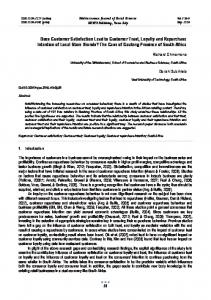
Figure 2. A recursive model for how value depends on support and hardware. All three of these variables are latent, and are estimated using measurement models having three, four, and five indicator variables, respectively. The indicators are in squares and have arrows point to their respective LVs. Each indicator has associated with it a measurement error named as a single letter and digits, e.g. s1. Each of these is drawn in a circle since they are unobserved. The curved, two headed arrow between support and hardware is a covariance. It represents an association that isn’t directional, unlike the paths from hardware and support to value. This model is essentially a regression model in LVs that has two predictors that are correlated. 1998 Sawtooth Software Conference ©1999 LBA: Lynd Bacon & Associates, Ltd. All Rights Reserved - 17 -

e1

e2

e3

e4

e5

e6

e7

e8

p1

p2

p3

p4

s1

s2

s3 .68

s4

.76

.68 .72

.66

.80

.51

.85

.66

satisfaction

performance

zeta Figure 3. Path diagram showing standardized coefficient estimates for a CSM fit using AMOS 3.61. The variance-covariance matrix of the observed variables p1…s4 was analyzed. The variables p1 through p4 are the indicators for the LV performance. s1 through s4 are the indicators for the satisfaction LV. Zeta is a regression error. The coefficients labeling paths from the LVs to the observed variables are estimates of standardized factor loadings. The unobserved variables e1 through e8 are sources of variation unique to the observed variables they point to. The coefficient on the path between performance and satisfaction is the standardized regression coefficient for performance. N=200.

e1

e2

e3

e4

e5

e6

p1

p2

p3

p4

s1

s2

.76

.68 .72

.51

.79 .81 .63 .82 performance

.80

.85

.66

.85 .76

e7

e8

s3

s4

.68

.66

.77 .76

satisfaction

.68 zeta

Figure 4. PLS coefficients shown in larger fonts from analysis of the correlation matrix of the observed variables p1…s4. The quantities in smaller font are standardized estimates from the CSM model shown in Figure 3. The diagram is otherwise labeled like Figure 3.

1998 Sawtooth Software Conference ©1999 LBA: Lynd Bacon & Associates, Ltd. All Rights Reserved - 18 -

Table 1. Basic specifications for covariance structure and PLS models. The basic CSM structural model expresses the relationship between endogenous LVs tercepts α , regression coefficients

η , in-

Β and Γ , exogenous LVs ξ , and errors in equations ζ .

η = α + Βη + Γξ + ζ Where η , ξ , α , and ζ are vectors, and Β and Γ are matrices. CSM measurement models connect observed indicator variables Y for endogenous LVs, and observed indicators X for exogenous LVs:

Y = Λ Yη + ε X = Λ Xξ + δ The matrices Λ contain factor loadings for the observed variables on the LVs, and ε , δ are "uniquenesses," i.e. sources of variance other than the LVs. Their expected values are assumed to be zero. Intercepts may also be included in the measurement models. A complete CSM specification includes covariance matrices for the various kinds of errors and for the exogenous LVs. PLS has inner and outer models. The PLS inner model can be expressed as:

η = α + Βη + Γξ + ζ Where the LVs in

η

1 6

can be ordered such that

1 6

Β is lower diagonal.

Assumptions include

E ζ = 0 , cov ζ , η = cov ζ , ξ = 0 . The outer model for reflective indicators is:

Y = Λ Yη + ε Y X = Λ Xξ + ε X And for formative indicators:

η = ΠY Y + δ η ξ = ΠX X +δξ The

Λ

are loadings and the

Π are regression coefficients. The expected values of the

are zero, and they are assumed to not covary with

η, ξ .

1998 Sawtooth Software Conference ©1999 LBA: Lynd Bacon & Associates, Ltd. All Rights Reserved - 19 -

ε ,δ

The PLS specification also includes weights that are used to estimate the scores on predicted values are obtained as, e.g.

η, ξ .

The

ξ$ = ∑ wx , and how the weights w are determined de-

pends on the kind of outer model used for each LV as well as the LVs role in the inner model.

1998 Sawtooth Software Conference ©1999 LBA: Lynd Bacon & Associates, Ltd. All Rights Reserved - 20 -

Table 2. Short comparison of CSM and PLS Characteristics Feature CSM PLS Distribution assumptions

Observed variables are MVN for ML, GLS estimation. Independent observations.

None

Continuously distributed observed variables for ADF/WLS. Types of models that can be fit Types of observed variables

Recursive, non-recursive Continuous Ordered discrete (using polychoric correlations as input, assuming robustness, or using the LISCOMP specification.

Recursive Continuous Ordered and unordered discrete

Type of latent variables that can be modeled Types of indicators for latent variables

Continuous

continuous

Effect- arrow from LV to indicator Causal- arrow from indicator Must be considered. Heuristics are available for common model forms. Otherwise, empirical procedures are required Can be as few as one if the indicator’s error is constrained. Otherwise, the number depends on parameter identification requirements. An observed variable can indicate more than one LV Yes

reflective, formative (analogous to effect and causal indicators, respectively) Not an issue for standard PLS models.

Yes

no

Yes

No

Simultaneous estimation of parameters by minimizing discrepancies between observed and predicted VCV matrix (or correlation matrix). Full information methods.

Multi-stage iterative procedure using OLS. Model is divided into blocks whose parameters are estimated separately. A limited information method.

Identification of parameters

Effects indicators per factor

Factors per indicator Correlation between LVs can be estimated as undirected Correlation between measurement errors can be modeled Estimation of means and intercepts on LVs Type of Fitting algorithm

One or more, but see "Consistency of estimators"

Observed variables can only indicate one LV No

1998 Sawtooth Software Conference ©1999 LBA: Lynd Bacon & Associates, Ltd. All Rights Reserved - 21 -

Feature Consistency of estimators

Availability of statistical tests for estimates

Measures of fit

Assessing measurement model quality

Sample size requirements

Factor indeterminancy

2nd-order factors can be modeled Estimation of random coefficients Latent class/finite mixture modeling Missing data

Table 2. (continued) CSM Consistent, given correctness of model and appropriateness of assumptions

Available and valid given key model assumptions are tenable. Inference by bootstrapping, otherwise. A great variety of them. Distributional theory worked out for some, not for others. Some allow inferences about nested models. Measures for assessing reliability and validity are available that permit observed variables to indicate more than one LV Larger than for multiple regression. Procedures for estimating required N and for power analysis are available. Latent variable scores are not estimated directly. Scale of measurement for each factor must be set using a constraint. Yes

PLS "Consistency at Large:" Estimates become consistent when the sample size gets large, and the number of indicators/LV gets large. Inference requires jacknifing or bootstrapping.

Coefficient of determination for 2 each equation, Q predictive relevance measures. Can be used for nested model comparisons with bootstrapping. Measures of reliability and validity are available.

Small to moderate. A heuristic is to use 10-20 observations per parameter in the largest model block. See "consistency of estimators." None. Latent variable scores are estimated as exact linear combinations of observed variables. Yes

yes, for some model types

No

Yes, for some model types

no

Algorithms assume complete data, but imputation can be done w/in some available SEM software packages.

Assumes complete data. Imputation using other software.

1998 Sawtooth Software Conference ©1999 LBA: Lynd Bacon & Associates, Ltd. All Rights Reserved - 22 -