USING MODIFIED FUZZY PARTICLE SWARM OPTIMIZATION ...

International Journal of Innovative Computing, Information and Control Volume 8, Number 1(B), January 2012

c ICIC International ⃝2012 ISSN 1349-4198 pp. 567–581

USING MODIFIED FUZZY PARTICLE SWARM OPTIMIZATION ALGORITHM FOR PARAMETER ESTIMATION OF SURGE ARRESTERS MODELS Mehdi Nafar1 , Gevork B. Gharehpetian2 and Taher Niknam3 1

Department of Electrical Engineering Science and Research Branch Islamic Azad University Tehran, Iran [email protected] 2

Electrical Engineering Department Amirkabir University of Technology Tehran, Iran [email protected]

3

Department of Electrical and Electronic Engineering Shiraz University of Technology Shiraz, Iran [email protected]

Received September 2010; revised January 2011 Abstract. Accurate modeling and parameters identification of Metal Oxide Surge Arrester (MOSA) are very important for arrester allocation, systems reliability and insulation coordination studies. Several models with acceptable accuracy have been proposed to describe this behavior. It should be mentioned that the estimation of nonlinear elements of MOSAs is very important for all models. In this paper, a new method, which is the combination of Fuzzy Particle Swarm Optimization (FPSO) and Ant Colony Optimization (ACO) methods, is proposed to estimate the parameters of MOSA models. The proposed method is named Modified Fuzzy Particle Swarm Optimization (MFPSO). In the proposed algorithm, to overcome the drawback of the PSO algorithm (convergence to local optima), the inertia weight is tuned by using fuzzy rules. Also, to improve the global search capability and prevent the convergence to local minima, ACO algorithm is combined to proposed FPSO algorithm. The transient models of MOSA have been simulated by using ATP-EMTP. The results of simulations have been applied to the program, which is based on MFPSO method and can determine the fitness and parameters of different models. The validity and the accuracy of the estimated parameters are assessed by comparing the predicted residual voltage with the experimental results. Also, Using proposed algorithm, different surge arrester models and V-I characteristics determination methods have been compared. Keywords: Surge arrester models, PSO, ACO, Fuzzy rules, Parameter estimation

1. Introduction. MOSAs are widely used as protective devices against lightning and switching over-voltages. Accurate modeling and simulation of their dynamic characteristics is very important for arrester allocation, systems reliability and insulation coordination studies [1-7]. For switching surge studies, MOSAs can be modeled by their nonlinear V -I characteristics [1,2]. However, such a presentation would not be appropriate for fast front transient and lightning surge studies. Because the MOSA shows dynamic characteristics such that the voltage across the surge arrester increases as the time-to-crest of the arrester current decreases and the voltage of arrester reaches a peak before the arrester 567

568

M. NAFAR, G. B. GHAREHPETIAN AND T. NIKNAM

current peaks [6]. Typically, the residual voltage of an impulse current having a front time equal to 1 µs is 8-12% higher than that predicted for an impulse current having a front time equal to 8 µs. The residual voltage of a longer time-to-crest between 45 and 60 µs, is 2-4% lower than that of a 8 µs current impulse [6]. In order to reproduce the MOSA dynamic characteristics, many studies have been focused on modeling and simulation of MOSAs [1-6]. In [1], a dynamic model has been presented by IEEE, which is based on database for fast impulse currents (time-to-crest of 0.5-45 µs). The IEEE model has been simplified and changed to other models by other researchers [2,3]. The main problem of these models is essentially their parameters calculation and estimation [1-7]. It should be noted that the determination of nonlinear resistors of MOSA is very important for the proposed models. These resistors could be presented by voltage-current tables given in [1]. Also, the voltage-current characteristic of a nonlinear resistor could be presented by an exponential equation [6]. In this paper, the combination of algorithms has been proposed to determine the best parameters for MOSAs models. One of the evolutionary algorithms that have shown great potential and good perspective for the solution of various optimization problems is Particle Swarm Optimization (PSO) [8]. The PSO algorithm was developed through simulation of a simplified social system such as social behavior of birds flocking or fish schooling [8]. PSO has been found to be robust in solving continuous nonlinear optimization problems. However, the performance of the standard PSO greatly depends on its parameters, such as inertia weight, cognitive and the social parameters, and it often suffers from the problem of being trapped in the local optima. Eiben et al. [11] described two ways of defining the parameter values: adaptive parameter control and self-adaptive parameter control. In the former, the parameter values change according to a heuristic rule that takes feedback from the current search state, while in the latter, the parameters of the meta-heuristic are incorporated into the representation of the solution. Thus, the parameter values evolve together with the solutions of the population. In this paper, an adaptive parameter control is used for inertia weight using a fuzzy logical controller. Also, in order to avoid trapping in local optima, Ant Colony Optimization (ACO) algorithm is combined to Fuzzy PSO (FPSO) to explore the search space much more efficiently. Using the proposed algorithm and linking the MATLAB and EMTP programs, parameters of MOSA models are estimated. Based on the estimated parameters, the models have been simulated and then the results of simulations have been compared with the experimental results. The results show the ability of the proposed algorithm in determining the surge arrester parameters. Also, using proposed algorithm, different surge arrester models and V -I characteristics determination methods have been compared. The main contributions of this paper are as follows: (i) Present a new method for parameters estimation of all surge arrester models without the need for the formulation, equation and information on the surge arrester dimensions. (ii) Present a new modified evolutionary optimization algorithm based on PSO and ACO algorithms and fuzzy rules. (iii) Apply the proposed optimization algorithm on parameter estimation of surge arrester problem by using a new method for linking the MATLAB and EMTP programs. 2. Surge Arresters Modeling. The transient models of MOSAs are necessary for insulation coordination and reliability studies of power systems. Several surge arrester models have been proposed to describe the transient behavior of surge arresters [1-3]. In this paper, transient models are investigated in the following text. The model, shown in Figure 1, has been suggested by IEEE WG 3-4-11 group [1]. As it is shown in this figure, the nonlinear V -I characteristics has been modeled by two

USING MODIFIED FPSO ALGORITHM FOR PARAMETER ESTIMATION

569

nonlinear resistors A0 and A1 which are separated by a RL low pass filter. The calculation of parameters of this model has been presented in [4]. It is based on the estimated height of the arrester column, the number of columns of MO disks and Table 1. Table 1. V -I characteristics for A0 and A1 (V10 is the discharge voltage (in kV) for a 10 kA, 8/20 µs current) Current (kA) 0.01 0.1 1 2 4 6 8 10 12 14 16 18 20

Voltage (per unit of V10 ) A0 A1 0.875 – 0.963 0.769 1.050 0.850 1.088 0.894 1.125 0.925 1.138 0.938 1.169 0.956 1.188 0.969 1.206 0.975 1.231 0.988 1.250 0.994 1.281 1 1.313 1.006

Figure 1. IEEE model The model, shown in Figure 2, has been proposed by Pinceti [2]. The parameters calculation procedure for this model has been presented in [2].

Figure 2. Pinceti model In [3], Fernandez et al. have presented another model which is based on IEEE model too. This model is shown in Figure 3. An iterative trial and error procedure has been proposed in [3], to determine the model parameters.

570


Figure 3. Fernandez model The identification of nonlinear parts of MOSAs is important for the proposed models. The voltage-current characteristics of a nonlinear resistor can be directly expressed by Equation (1) [6]. I = p (V /V ref )q (1) where p and q are constant values, V and I are voltage and current of surge arrester, respectively, and Vref is an arbitrary reference voltage. For the models based on IEEE model, the initial nonlinear V -I characteristics values of A0 and A1 could be determined by Table 1 [1,4-6]. The procedures mentioned above, do not always result in the best parameters, but they can provide a good estimation (a starting point) [1-6]. It should be noted that these methods are limited to mentioned models. In recent years, several researches have been presented for estimating the parameters of all models [5,6]. A numerical method has been proposed for identifying the parameters of three suggested models in [5]. This method is based on comparison of the simulation results of residual voltages and the results derived from 8/20 µs experimental measurements [5]. In this method, parameters of surge arrester models are estimated by minimizing the following objective function: ∫ T F = W (t) [V (t, x) − V m(t)]2 dt (2) 0

where F is sum of the quadratic error, T is duration of applied impulse current signal, V (t, x¯) is the estimated residual voltage obtained from simulation results, V m(t) is the measured voltage, x¯ is the state variable vector (surge arrester model parameters) and W (t) is the weighting function, derived from numerical experimentation. In this method, the non-linear resistances have been presented by piecewise functions and consequently a linearization has been adopted. The problem of optimization has been solved in two stages with an aim of avoiding possible numerical oscillations of the predicted voltage. In this paper, a new method based on heuristic algorithms is suggested to estimate the best parameters of MOSAs models. Proposed method is general and can be applied to all surge arrester models. Unlike existing procedures, equation or formulation and information on the surge arrester dimensions are not necessary. Also, the application of the weighting function is not necessary in suggested method and the non-linear resistors can be represented based on Equation (1) or based on Table 1. Also, using proposed algorithm, nonlinear characteristics of surge arrester are estimated via Equation (1) and then they are compared with the results of the IEEE method (using Table 1). 3. Objective Function. The ATP-EMTP software has been used as the simulation tool. The 8/20 µs impulse current is applied to the simulated models of surge arresters. The simulated residual voltage of each model is compared with the experimental data obtained


from [7]. The comparison method is based on Equation (3), as follows: ∫ T F = [V (t, x¯) − V m(t)]2 dt

571

(3)

0

This objective function can be rewritten in the discrete form, as follows: F =

N ∑

[V (j∆t, x) − Vm (j∆t)]2 ∆t

(4)

j=1

where N is the number of discrete points and the ∆t = T /N is computation time step. The parameters of surge arrester Models (¯ x), determined by proposed algorithm in MATLAB, are imported to the EMTP. In this paper, the simulation is carried out by using the 10 kA, 8/20 µs impulse current. The chosen step time in simulation is 0.5 µs. So, the residual voltage vector of each model (V (t, x¯)) is determined by EMTP and then is compared with the measured voltage vector (V m(t)). The objective function is evaluated and minimized by using the proposed algorithm and the best parameters of surge arrester models (¯ x) are estimated. 4. Algorithm of Optimization. 4.1. ACO algorithm. Since ants are blind insects, which live together, they find the shortest path from the nest to the food with the aid of pheromone. A chemical material deposited by the ants, pheromone serves as a critical communication facility among ants which help them in their path recognition. Pheromone intensity deposited by ants determines the shortest path in their way to food. Generally, the state transition probability to select the next path can be expressed, as follows: (τij )γ2 (1/Lij )γ1 Pij = N A (5) ∑ γ2 γ1 (τij ) (1/Lij ) j=1,j̸=i

After choosing the next path, updating the trail intensity of pheromone is as: τij (k + 1) = ρτij (k) + ∆τij

(6)

where τij is the intensity of pheromone between the nodes j and i, Lij is the length of path between the nodes j and i, γ1 is the control parameter for determining the weight of trail intensity, γ2 is the control parameter for determining the weight of the length of path, N A is the number of ants, ρ is a coefficient such that (1 − ρ) represents evaporation of trail between time k and k + 1 and ∆τij is the amount of pheromone trail added to τij by ants. 4.2. Standard PSO algorithm. PSO is a population based stochastic optimization algorithm, inspired by social behavior of bird flocking or fish schooling, developed by Eberhart and Kennedy. It is a useful technique to solve many optimization problems [8-10]. PSO shares many similarities with evolutionary computation techniques such as Genetic Algorithms (GA). The system is initialized by a population of random solutions and searches for optima by updating generations. However, unlike GA, PSO has no evolution operators such as crossover and mutation. In PSO algorithm, the potential

572


solutions, called particles, fly through the problem space by following the current optimum particles. Equation (7) could describe the content of this concept. ( ) ( ) (t) (t) (t+1) (t) Vi = ω.Vi + c1 .rand1 (.). P besti − Xi + c2 .rand2 (.). Gbest − Xi (7) (t+1) (t) (t+1) Xi = Xi + Vi where rand1 (.) and rand2 (.) are random number between 0 and 1, Pbest is best previously recorded experience of the ith particle, Gbest is best particle among the entire population and the constants c1 and c2 are weighting coefficients of the stochastic acceleration terms which stimulate each particle towards Pbest and Gbest positions. Low values allow particles to go far from the target region [13,14]. The coefficients c1 and c2 are often set to 2.0 according to previous experiences [8-10]. The appropriate selection of inertia weight ω in Equation (7) provides a proper global and local search as it is essential to minimize iteration average to achieve a sufficient optimal solution. Approximately the coefficient ω often decreases linearly from 0.9 to 0.4 during a run. Generally, Equation (8) could present the inertia weight ω as follows: ωmax − ωmin ω (t+1) = ωmax − ×t (8) tmax where ωmax and ωmin are maximum and minimum of the inertia weight, respectively, and tmax is maximum number of iterations. 4.2.1. Fuzzy adaptive inertia weight factor. In PSO, the search process is a nonlinear and dynamic procedure. Therefore, when the environment itself is dynamically changed over the time, the optimization algorithm should be able to adapt dynamically to the changing environment. The change of the particle’s situation is directly correlated to the inertia weight. Proper choice of the inertia weight ω provides a balance between global and local optimum points [10]. Several methods have been applied to handle the inertia weight during the progression of the optimization process. Constant inertia weight, linearly decreasing inertia weight and random inertia weight are some examples [12,13]. In this paper, a fuzzy IF/THEN rules is used to adaptively control the inertia weight of PSO. Four steps are taken to create the fuzzy system: fuzzification, fuzzy rules, fuzzy reasoning and defuzzification. These steps are described in the following subsections. (1) Fuzzification. The fuzzification comprises the process of transforming crisp values into grades of membership for linguistic terms of fuzzy sets [14]. For each input and output selected variable, two or more membership functions are described. Normally, they are three but can be more. In this paper, among a set of membership functions, left-triangle, triangle and right triangle membership functions are used for every input and output as shown in Figure 4. All the memberships of input are presented in three linguistic levels; S, M and L for small, medium and large, respectively in Table 2. The output variable has been presented in three fuzzy sets of linguistic values; NE (negative), ZE (zero) and PE (positive) with associated membership functions, as shown in Figure 4 [12]. (2) Fuzzy rules. The fuzzy rules are a series of IF-THEN statements. These statements are usually derived by an expert to achieve optimum results. In this paper, the Mamdani-type fuzzy rules have been used to evaluate the conditional statements that comprise fuzzy logic. For example: if (NFV is L) and (ω is M) THEN (∆ω is ZE), where NFV is normalized fitness value and NFV is an input variable between 0 and 1. The fuzzy rules of Table 2 are used to select the inertia weight correction (∆ω). Each rule represents a mapping from the input space to the output space. (3) Fuzzy reasoning. In this paper, Mamdani’s fuzzy inference method is used to map the inputs to the outputs. The AND operator is used for the combination of membership


(a)

(b)

573

(c)

Figure 4. Membership functions of inputs and outputs: (a) NFV, (b) ω and (c) ∆ω Table 2. Fuzzy rules for variations of inertia weight ∆ω NFV

ω S M L

S ZE PE PE

M NE ZE ZE

L NE NE NE

values for each fired rule to generate the membership values for the fuzzy sets of output variables in the consequent part of the rule. Since there may be several rules fired in the rule sets for some fuzzy sets of the output variables there may be different membership values obtained from different fired rules. To obtain a better inertia weight under the fuzzy system, the current best performance evaluation and current inertia weight are selected as inputs variables; where as the output variable is the change in the inertia weight. The NFV is used as an input variable between 0 and 1, and is defined as: F V − F Vmin NF V = (9) F Vmax − F Vmin In the first iteration, the calculated value of F V may be selected as F Vmin for the next iterations. In Equation (9), F Vmax is the worst solution for the minimization process. Typical inertia weight value is in range of 0.4-0.9. Both positive and negative corrections limits are required for the inertia weight. Therefore, a range of [−0.1 0.1] has been chosen for the inertia weight correction. ω t+1 = ω t + ∆ω

(10)

In order to choose an appropriate representative value as the final output (crisp values), defuzzification must be done. It will be illustrated at a later point. (4) Defuzzification. In order to obtain a crisp value, the output must be defuzzyfied. For defuzzification of every input and output, the method of centroid (center-of-sums) has been used for the membership functions as shown in Figure 4. 4.3. Proposed MFPSO algorithm. The PSO method should be considered as a useful method, which is powerful enough to handle various kinds of nonlinear optimization problems. Nevertheless, it may be trapped into local optima, if over a number of iterations, global best and local best positions are equal to the position of the particle. Recently, numerous ideas have been used to overcome this drawback using other global optimization algorithms such as Evolutionary Programming (EP), Genetic Algorithm (GA) or

574


Simulated Annealing (SA) along with the PSO [9]. The performance of the standard PSO greatly depends on its parameters, such as inertia weight, cognitive and the social parameters, and it often suffers from the problem of being trapped in the local optima. In this paper, an adaptive parameter control is used for inertia weight by using a fuzzy logical controller. Also, in order to avoid trapping in local optima, ACO algorithm is combined to FPSO to explore the search space much more efficiently. This new algorithm proposes the application of the intelligent decision-making structure of ACO algorithm to the APSO algorithm such that a unique global best position is obtained for each particle. However, it uses random selection procedure of ACO algorithm to determine different global best positions of each distinct agent. This algorithm, called Modified Fuzzy Particle Swarm Optimization (MFPSO) is used to minimize the cost function of the surge arrester parameters estimation problem. The proposed MFPSO algorithm has the following steps: Step 1: Generate the initial population and initial velocity. The initial population and initial velocity of each particle are randomly generated, as follows:   x1   x2  , xi = [xi ] P opulation =  1×n   ... (11) xNSwarm min xi = rand(.) × (xmax − xmin i i ) + xi   V1   V2  , Vi = [vi ] V elocity =  1×n   ... VNSwarm

(12)

vi = rand(.) × (vimax − vimin ) + vimin where NSwarm is the number of the swarms, n is the number of the state variable, xmax and xmin are the maximum and minimum of ith state variable, respectively i i max and vi and vimin are the maximum and minimum velocity of ith state variable. Step 2: Generate the initial trail intensity. In this initialization phase, it is assumed that the trail intensity between each pair of swarms is the same and is generated, as follows: T rail Intensity = [τij ]NSwarm ×NSwarm , Step 3:

Step 4:

Step 5:

Step 6: Step 7:

τij = τ0

(13)

where τ0 is the initial trial intensity. Coupling to EMTP. The surge arrester model is simulated by EMTP using the given data (parameters). Then, the simulation results are transferred to the MFPSO-based developed program to calculate the objective function. Calculate the objective function. The objective function (i.e., Equation (4)) is calculated for each individual by using the simulation results obtained in Step 3. Sort the initial population. In this step, the initial population is sorted in ascending order considering the value of the objective function of each individual. Select the best global position. The individual that has the minimum value of the objective function is selected as the best global position (i.e., Gbest). Select the best local position. The best local position (Pbest) is selected for each individual.


575

Step 8: Update the parameters. In this algorithm, the proper choice of inertia weight, ω, is updated by the fuzzy rules. Step 9: Select the ith individual. The ith individual is selected and neighbors of this particle should be dynamically defined as follows:             1   ( )  , i ̸= j Si = xj | ∥xi − xj ∥ ≤ 2D0  (14)   −at     1 − exp tmax where D0 is the initial neighborhood radius and a is the parameter used to tune the neighborhood radius. Step 10: Calculate the next position for the ith individual. There are two approaches to calculate the next position, as follows: • Approach A) if Si ̸= {}, where {} stands for the null set In this case, the transition probabilities between xi and each individual in Si are calculated by the following equation: [P robability]i = [Pi1 , Pi2 , . . . , Pi,M ]1×M , (τij )γ2 (1/Lij )γ1 Pij = M , ∑ γ2 γ (τij ) (1/Lij ) 1

Lij =

1 |F (xi ) − F (xj )|

(15)

j=1

Then, the cumulative probabilities are calculated as follows: [Cumulative probability]i = [C1 , C2 , . . . , CM ]1×M

(16)

C1 = Pi1 , C2 = C1 + Pi2 , . . . , Cj = Cj−1 + Pij , . . . , CM = CM −1 + PiM where M is the number of members in Si and Cj is the cumulative probability for the j th individual in Si . The roulette wheel is used for the stochastic selection of the best global position, as follows: A number between 0 and 1 is randomly generated and is compared with the calculated cumulative probabilities. The first term of the cumulative probabilities (Cj ), which is greater than the generated number, is selected and the associated position is considered as the best global position. Then, the ith particle is moved according to following rules, if xj is selected as the best: ) (  (t+1) (t) (t)  x V = ω.V + c .rand (◦). P best − 1 1 i  i i i   ( ) (t) (17) + c2 .rand2 (◦). xj − xi     (t+1) (t+1) (t) = xi + Vi xi The presumed pheromone level between Xi and Xj is updated in the next stage: τij (t + 1) = ρ.τij (t) + Pij

(18)

• Approach B) if Si = {}, which means there is not any individual in particle’s neighborhood.

576


In this case, the ith particle is moved according to the following rules: ( )  (t+1) (t) (t)  V = ω.V + c .rand (◦). P best − x 1 1 i  i i i   ( ) (t) (19) + c2 .rand2 (◦). Gbest − xi     (t+1) (t) (t+1) xi = xi + Vi Then, the trail intensity is updated as follows: τij (t + 1) = ρ.τij (t) + r;

0.1 ≤ r ≤ 0.5

(20)

where index j represents the best particle index in the group. The modified position for the ith individual is checked with its limit. Step 11: If all individuals have been selected, go to the next step, otherwise, i = i + 1 and go back to Step 5. Step 12: Check the termination criteria. If the current iteration number reaches the predetermined maximum iteration number, the search procedures should be stopped; otherwise the initial population is replaced by the new population of swarms and then the algorithm goes back to Step 3. The last Gbest is the solution of the problem. 5. Link between EMTP and MATLAB. Both ATP-EMTP and MATLAB are currently available on popular computer for engineering applications. It could be said that the best optimization algorithms can be easily developed in MATLAB and transient models of power system elements can be simulated by ATP-EMTP. To use the ability of both soft wares, a link between these programs is necessary. In [16], several techniques for link between EMTP and MATLAB have been presented, where MATLAB functions can be called in EMTP. However, in this paper, ATP files have been called as an input file of MATLAB. This approach is much easier than the other one. The surge arrester parameters have been estimated by using MFPSO algorithm developed in MATLAB and the surge arrester models have been simulated by EMTP [15]. A FORTRAN code file (ATP file) has been developed for each EMTP Simulation file. By using input/output functions of MATLAB, ATP file can be called in MATLAB and can be modified. So, the surge arrester parameters can be modified according to MFPSO outputs. Using SYSTEM command, the modified ATP file can be run in MATLAB. After running the ATP file, a LIS file is generated which contains the simulation outputs of surge arrester models are in this file. Then, using input/output function, LIS file could be opened in MATLAB and the residual voltage of simulation could be returned to MFPSO algorithm in MATLAB. This procedure can be repeated. 6. Parameter Estimation of Surge Arrester Models. The surge arrester models have been simulated by ATP-EMTP. Equation (1) can be used to determine V -I characteristic of A0 and A1 in MOSA models. In this equation, three parameters (p, q and Vref f ) must be identified for each nonlinear resistor. According to data given in Table 1, V -I characteristics of A0 and A1 can also be determined. In this case, the first step of the simulation is multiplying the per unit values of voltages by V10 and then the coefficients (Vref f ) of A0 and A1 are selected such that the simulated voltage and the experimental results are approached. So, in this case, a Vref f must be determined for each nonlinear element. In this section, MOSAs parameters models (linear and nonlinear parameters) have been estimated by the suggested algorithm for models of [1-3]. The surge arrester parameters, estimated by MFPSO algorithm in MATLAB, are imported to the EMTP.


577

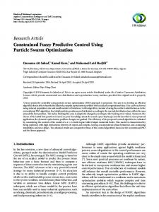
The simulation is carried out using the 10 kA, 8/20 µs impulse current. During optimization, the residual voltage of each model is determined by EMTP and then it is transferred to MFPSO algorithm in MATLAB to evaluate the fitness function. This procedure continues until the optimal solution is determined for parameters of that model. The residual voltage of simulations is compared to the experimental data given on [7]. The estimated parameters of all models, determined using Equation (1) and the experimental data of [7], are listed in Table 3. A comparison among experimental and the simulated residual voltage obtained by estimated parameters of the models of [1-3] based on Equation (1) is shown in Figure 5.

Figure 5. Comparison between measured and simulated results based on Equation (1) Table 3. Estimated parameters (using Equation (1)) parameter Model of [1] Model of [2] Model of [3] R0 (Ω) 0.0870 12.515 7.22 R1 (Ω) 0.7789 – – L0 (µH) 0. 4239 0.065 – L1 (µH) 0. 0612 0.998 0.8969 C (nF ) 1.9392 – 9.01 p0 3410.35 3129.32 3094.26 q0 16.3007 9.01 12.32 p1 4137.82 2574.62 6199.99 q1 6.5868 15.18 19.19 V ref f0 [V ] 7846.85 7579.95 7909.69 V ref f1 [V ] 7278.82 7602.89 7811.48 According to the results of [7], the nonlinear V -I characteristics of A0 and A1 for the models of [1-3] have been estimated by using the data of Table 1. The results have been listed in Table 4. The residual voltages determined by estimated surge arrester models and measured by [7] have been shown in Figure 6.

578


Table 4. Estimated parameters (using data of Table 1) parameter Model of [1] Model of [2] Model of [3] R0 (Ω) 0.405 9.8 5.6 R1 (Ω) 0.326 – – L0 (µH) 0.0446 0.0069 – L1 (µH) 1.0656 0.6589 0.693 C (nF ) 0.0783 – 0.270 V ref f0 [V ] 7380.05 7417.29 7515.69 V ref f1 [V ] 7403.67 7640.49 7579.15

Figure 6. Comparison between measured and simulated results based on Table 1 Comparing Figures 5 and 6, it can be seen that V -I characteristics of nonlinear parts of all surge arrester models can be determined by both methods. As it can be seen in this figure, the simulation results have a good agreement with the experimental data. As it could be seen in these figures, for IEEE model, the result obtained by Equation (1) is more accurate than the IEEE method, especially for the end part of the curve. It should be said that both methods are accurate enough for insulation coordination studies. However, the model according to Equation (1) can determine the energy absorption of surge arrester better than the IEEE method. For the Pinceti model, both methods are accurate enough but for the Fernandez model, the model based on Equation (1) has a better agreement with experimental data. It should be noted that, using proposed method, parameters of all surge arrester models could be properly estimated. 7. Error Analysis. In [7], measurements were performed to get the response of surge arrester block for two types of impulse currents. These currents are steep front wave impulse (1/2 µs) and standard impulse (8/20 µs) impulse currents. The peak values of impulse currents were changed in each impulse test. The peak values of measured residual voltages of arrester block for these impulses are presented in Tables 5 and 6. In this section, using these experimental data, the ability of the proposed method to estimate the parameters of surge arrester models and the ability of models to simulate


579

the arrester dynamic behavior are presented. The models of [1-3], have been simulated in EMTP based on the estimated parameters of Tables 3 and 4. The current peak values in simulation are 2.5 kA, 5 kA and 10 kA and the selected rise and fall times are 1/2 µs and 8/20 µs. The 1/2 µs impulse current has been applied to the models and the simulation results have been used to determine the error by the following equation: Vsim − Vmeas × 100 (21) Vmeas where Vsim and Vmeas are the peak values of simulated and measured residual voltage, respectively. The results of this calculation have been presented in Table 5. The same simulations and calculations have been repeated for 8/20 µs impulses. The results are presented in Table 6. In these tables, P.C. and P.V. stand for “peak of impulse current” and “peak of measured residual voltage”, respectively. According to the results of these tables, the following points could be drawn: • The surge arrester models based on the data of table1 are more accurate in comparison with the models based on Equation (1); • All surge arrester models simulate the dynamic behavior of MOSA properly; • The suggested procedure can be applied to all surge arrester models and; • The proposed algorithm (MFPSO) is a powerful tool for identifying parameters of all surge arrester models. Error% =

Table 5. Comparison between measured and simulated results 1/2 µs impulse current Based on Equation (1) Based on data of Table 1 Models Peak of Residual Error % Peak of Residual Error % IEEE 6.869 –4.9 7.5978 1.84 P.C. = 2.58 kA Fernandeze 7.2571 –2.72 7.5181 0.77 P.V. = 7.46 kV Pinceti 7.0806 –3.08 7.6161 2.09 IEEE 7.6692 –3.7 8.0612 1.14 P.C. = 5.04 kA Fernandeze 7.8807 –1.12 8.0711 1.26 P.V. = 7.97 kV Pinceti 7.8106 –2 8.0718 1.27 IEEE 8.6914 0.82 8.6927 0.84 P.C. = 10.48 kA Fernandeze 8.5250 –1.10 8.7949 2.02 P.V. = 8.62 kV Pinceti 8.772 1.76 8.7598 1.62

8. Conclusions. In this paper, a new algorithm based on the combination of Fuzzy particle swarm optimization (FPSO) and ant colony optimization (ACO) has been proposed to improve the performance of PSO algorithm. In this proposed algorithm, known as MFPSO, to overcome the problem of the premature convergence observed in many applications of PSO, the inertia weight has been tuned by using fuzzy rules. Also, to improve the global search capability and prevent the convergence to local minima, ACO algorithm has been combined to proposed FPSO algorithm. A new method based on the MFPSO algorithm, and linking the MATLAB and EMTP programs has been proposed to estimate the parameters of MOSA models. Using the proposed algorithm, the parameters are estimated based on the MOSA residual voltage measurements. Also, using MFPSO algorithm, a comparative study among different methods of the surge arrester nonlinear V -I characteristics modeling has been conducted in this paper. It is show that the result obtained by using Equation (1) is more accurate for energy absorption studies of surge

580


Table 6. Comparison between measured and simulated results 8/20 µs impulse current Based on Equation (1) Based on data of Table 1 Models Peak of Residual Error % Peak of Residual Error % IEEE 6.7071 –4.32 7.3218 4.44 P.C. = 2.50 kA Fernandeze 7.0433 0.4750 7.0435 0.47 P.V. = 7.01 kV Pinceti 6.9138 –1.37 7.2492 3.41 IEEE 7.3922 –1.31 7.6871 2.63 P.C. = 5.01 kA Fernandeze 7.5126 0.30 7.5972 1.43 P.V. = 7.49 kV Pinceti 7.4821 –0.11 7.6635 2.31 IEEE 8.1103 0.38 8.1396 0.73 P.C. = 10.23 kA Fernandeze 8.0983 0.22 8.0966 0.21 P.V. = 8.08 kV Pinceti 8.1269 0.58 8.1083 0.35 arrester. However, the IEEE method (for V -I characteristics determination) is more accurate for insulation coordination studies. Also, it is shown that the estimated parameters of all models in the simulation results are in a good agreement with the residual voltage measurements. It should be noted that the previous studies were limited to special models but the proposed algorithm is general and comparing with other algorithms, it can be easily implemented and its convergence speed is considerable. Acknowledgment. This work is partially supported by Islamic Azad University, Science and Research Branch, Tehran, Iran. The authors also gratefully acknowledge the helpful comments and suggestions of the reviewers, which have improved the presentation. REFERENCES [1] IEEE WG 3.4.11, Modeling of metal oxide surge arrester, IEEE Trans. on Power Delivery, vol.7, pp.302-309, 1992. [2] P. Pinceti and M. Giannettoni, A simplified model for zinc oxide surge arresters, IEEE Trans. on Power Delivery, vol.14, pp.393-398, 1999. [3] F. Fernandez and R. Diaz, Metal oxide surge arrester model for fast transient simulation, Proc. of the International Conference on Power System Transients, pp.144-149, 2001. [4] J. A. Martinez and D. W. Durbak, Parameter determination for modeling systems transients – Part V: Surge arrester, IEEE Trans. on Power Delivery, vol.20, no.3, pp.2073-78, 2005. [5] H. J. Li, S. Birlasekaran and S. S. Choi, A parameter identification technique for metal-oxide surge arrester models, IEEE Trans. on Power Delivery, vol.17, no.3, pp.736-41, 2002. [6] M. Nafar, G. B. Gharehpetian and T. Niknam, A new parameter estimation algorithm for metal oxide surge arrester, Journal of Electric Power Components and Systems, vol.39, no.7, pp.696-712, 2011. [7] I. Kim, T. Funabashi, H. Sasaki and T. Hagiwara, Study of ZnO arrester model for steep front wave, IEEE Trans. on Power Delivery, vol.11, pp.834-841, 1996. [8] J. Kennedy and R. Eberhart, Particle swarm optimization, IEEE International Conf. on Neural Networks, pp.1942-1948, 1995. [9] Z.-L. Gaing, Particle swarm optimization to solving the economic dispatch considering the generator constraints, IEEE Trans. on Power System, vol.18, pp.1187-1195, 2003. [10] Y. Shi and R. Eberhart, A modified particle swarm optimizer, Proc. of the IEEE World Congress on Computational Intelligence, pp.69-73, 1998. [11] A. E. Eiben, R. Hinterding and Z. Michalewicz, Parameter control in evolutionary algorithms, IEEE Transactions on Evolutionary Computation, vol.3, pp.124-141, 1999. [12] P. Bajpai and S. N. Singh, Fuzzy adaptive particle swarm optimization for bidding strategy in uniform price spot market, IEEE Trans. on Power System, vol.22, pp.2152-2160, 2007.


581

[13] C. C. Chiu, M. J.-J. Wu, Y.-T. Tsai, N.-H. Chiu, M. S.-H. Ho and H.-J. Shyu, Constrain-based particle swarm optimization (CBPSO) for call center scheduling, International Journal of Innovative Computing, Information and Control, vol.5, no.12(A), pp.4541-4549, 2009. [14] T. Wang, Y. Chen and S. Tong, Fuzzy improved interpolative reasoning methods for the sparse fuzzy rule, ICIC Express Letters, vol.3, no.3(A), pp.313-318, 2009. [15] Canadian/American EMTP User Group, Alternative Transients Program Rule Book, European EMTP Center, Leuven, Belgium, 1987. [16] J. Mahseredjian, G. Benmouyal and X. Lombard, A link between EMTP and MATLAB for userdefined modeling, IEEE Trans. on Power Delivery, vol.13, no.2, pp.667-674, 1998.