1. Using multivariate resultants. [22] to find the intersections of 3 implicit quadric surfaces is a new approach in CAGD.2 It provides new insight to the intersection.
Using Multivariate Resultants to Find the Intersection of Three Quadric Surfaces ENG-WEE
CHIONH
National University RONALD
of Singapore
N. GOLDMAN
Rice University and JAMES
R. MILLER
University
of Kansas
Macaulay’s
concise
but explicit
expression
for nmltivariate
resultants
has many
potential
applications in computer-aided geometric design. Here we describe its use in solid modeling for finding the intersections of three implicit quadric surfaces. By B6zout’s theorem, three quadric surfaces have either at most eight or intlnitely many intersections. Our method finds the intersections, when there are finitely many, by generating a polynomial of degree at most eight whose roots are the intersection coordinates along an appropriate axis. Only addition, subtraction, and multiplication are required to find the polynomial. But when there are pmsibilities of extraneous roots, division and greatest common divisor computations are necessary to identify and remove them. Categories and Subject Descriptors: 1.3.5 [Computer Graphics]: Computational Object Modeling– curve, surface and object representatwns; geometric algorithms, systems; physically based modeling General Terms: Algorithm,
Geometry and languoges and
Design, Theory
1. INTRODUCTION
Quadric surfaces appear with surprising regularity on the boundary of physical objects commonly modeled in computer-aided design and manufacturing (CAD/CAM) systems. However, only bounded portions of these surfaces actually lie on the boundary of the model. The challenge for computer-aided This work was supported by the National University of Singapore, by the National Science Foundation (NSF) under grant DMC-8813688, and by the University of Kansas under General Research allocation 3760-XO-0038. Authors’ addresses: E. W. Chionh, Department of Information Systems and Computer Science, National University of Singapore, Singapore; R. N. Goldman, Department of Computer EMence, Rice University, Houston, TX; J. R. Miller, Department of Computer Science, University of Kansas, 415 Snow Hall, Lawrence, KS 66045-2192. Permission to copy without fee all or part of this material is granted provided that the copies are not made or distributed for direct commercial advantage, the ACM copyright notice and the title of the publication and its date appear, and notice is given that copying is by permission of the Association for Computing Machinery. To copy otherwise, or to republish, requires a fee and/or specific permission. @ 1991 ACM 0730-0301/91/1000-0366 $01.50 ACM Transactions
on Graphics,
Vol. 10, No. 4, October
1991, Pages 378-400.
Using Multivariate Resultants to Find the Intersection
379
.
geometric design (CAGD) is to determine those portions of the surfaces that do lie on the object and to represent them in the database. Relevant portions of surfaces are generally determined from Boolean operations on quadric half-spaces. As a result, the pieces of the surfaces that lie on the model are bounded by curves of intersection between pairs of quadric surfaces. In general these curves are irreducible space quartics, although in certain situations they are reducible, either to a line plus a space cubic or to a pair of (possibly degenerate) conies. Like the surfaces from which they arise, it is typically the case that only portions of these curves actually lie on the boundary of the object. The endpoints of the curves are the locations in space where the complete curve intersects yet a third quadric surface. Computing the intersection curves and partitioning them at their intersections with other surfaces is one of the primary tasks of the Boundary Evaluation algorithm in solid modeling systems. This algorithm generates the boundary representation of the solid resulting from a Boolean operation applied to two other solids. Boundary evaluation is of vital importance to solid modeling systems since so many application functions and interaction techniques require a complete and accurate representation of the bounding faces, edges, and vertices of a solid. It is also generally the most complex piece of software in such systems, owing to the many complex geometric relationships that can arise which must be handled properly in an automatic fashion. The Boundary Evaluation algorithm operating on solids A and B can be summarized at a high level as follows [19]: 1. Generate
a suftlcient
(a) Intersect each boundary of B.
set of tentative surface
on
the
edges. boundary
of A with
each
surface
on
(b) Partition the original edges of A, the original edges of B, and the curves generated in part (a) at their intersections with other surfaces. 2. Classify each partitioned the resulting solid. 3. Retain
only
those
edges
edge whose
as INSIDE, classification
OUTSIDE,
or ON (the boundary
the new ofI
is ON.
Robust algorithms which address step l(a) in the context of the so-called natural quadrics have been described in Miller [13], O’Connor [17], and Piegl [181. General algebraic techniques not restricted to the natural quadrics are presented in Levin [81. Sarraga [21] has also studied these techniques in the context of the natural quadrics. Ocken et al. [16] have reported general algebraic intersection schemes applicable to any pair of rational surfaces (of which quadric surfaces are a subset). More recently, Farouki et al. [61have described general algebraic methods for automatically intersecting any pair of quadrics, detecting degenerate results such as conies and other rational parametric curve branches in the process. We focus in this paper on issues related to part (b) of step 1. At least 3 methods of partitioning curves are known. Since none of the methods perform satisfactorily (or are even applicable) in all situations, a given system will typically implement more than one technique and then use which ever one is best for a particular geometric configuration. Briefly, the known methods are the following (see Miller [12] for further details and references). ACM Trnasactions
on Graphics,
V.]
10, No. 4, October
1991
380
.
E.-W, Chionh et al.
(1) Curve-surfme intersection. Directly intersect the quadric surface intersection curve with other quadric surfaces on the model. This approach is commonly used when the curve is a straight line or a conic section. If an intersection curve between surfaces S1 (2) Curve-curve intersection. and S2 intersects (nontangentially) another surface S3, then it must be the case that both S1 and S2 intersect S3 along distinct intersection curves. The partitions could then be determined by intersecting any 2 of these 3 curves. Again this technique is most commonly employed when the two chosen curves are conic sections; however, Levin describes a rather elaborate algebraic scheme for intersecting two general nonplanar quartic intersection curves [8]. (3) Three-quadric intersection. It is clear from the discussion to this point that the bounding vertices of the curves lie at points common to three quadric surfaces. Partitioning the intersection curves by pursuing this observation is most commonly used as a fall-back approach when no two of the surfaces intersect in straight lines or conic sections. A scheme to find such points based on the application of quick heuristics with general, but slower, fall-back numerical methods is described in Morgan and Sarraga [141. The remainder of this paper describes a new approach using multivariate resultants to find the points in common to 3 quadric surfaces. 1 Using multivariate resultants [22] to find the intersections of 3 implicit quadric surfaces is a new approach in CAGD.2 It provides new insight to the intersection problem by isolating the algebraic details into a single resultant expression. At one stroke a polynomial of degree at most 8 is found, whose roots are the intersection coordinates along one of the coordinate axes. When the polynomial is a nonzero constant (degree zero), there is no intersection in affhe space; when it is identically zero, the intersection is infinite (a curve). We refer to such polynomials derived from resultants as intersection polynomials. Our method differs from those using the more commonly known Sylvester resultants [20]. With Sylvester resultants, an intersection polynomial can be found by successive elimination: first compute 3 resultants of degrees at most 4 by eliminating one variable; then compute 3 more resultants of degrees at most 16 by eliminating another variable; finally compute the greatest common divisor (GCD) of the latter 3 resultants. This method has several drawbacks. Computationally it is very expensive; 6 resultants and the GCD of 3 polynomials of degrees up to 16 must be computed. The degrees of the intersection polynomials produced may exceed 8, and more seriously, it is not clear how to detect and remove extraneous roots —roots which are introduced *While the curve and surface intersection techniques surveyed above, as well as the specific implementation of the 3 quadric intersection algorithms to be described, are applicable only to quadric surfaces, they are nonetheless useful in modeling systems supporting higher order surfaces, possibly in addition to quadrics. We expand upon two aspects of this observation in 8ection 6. ‘This use of multivariate resultants has also been discussed by Bajaj et al. [1]. ACM Transactions on Graphics, Vol. 10, No. 4, October
1991.
Using Multivariate Resultants to Find the Intersection
.
381
during the derivation of the intersection polynomial, but which do not represent the coordinates of any intersections. In contrast, multivariate resultants produce, in a single step, an intersection polynomial of degree at most 8. This approach also allows the identification of extraneous roots when they exist. In the following sections we briefly introduce resultants and describe Macaulay’s method3 for finding them. The use of multivariate resultants for computing the intersections of 3 implicit quadric surfaces is presented, and special techniques for practical implementation are discussed. These techniques include the avoidance of division in Macaulay’s multivariate resultant expression, systematic detection of degree deficiencies, and removal of extraneous roots. An evaluation of the accuracy and robustness of this method is also reported. 2. MACAULAY’S
MULTIVARIATE
RESULTANT
EXPRESSION
Resultants are an important tool in elimination theory. They are polynomial functions of the coefficients of a system of homogeneous (all terms having the same degree) polynomial equations, whose vanishing is a necessary and suficient condition for the system of homogeneous equations to have a nontrivial (not all zero) common solution. For k homogeneous polynomial equations in k variables, the resultant always exists. B6zout and Sylvester resultants are well-known resultant expressions for k = 2 (see Salmon, [20]). For k >2, a concise but explicit resultant expression was provided by Macaulay [10]. We use the term “multivariate resultants” for the case k >2, since in this case a resultant eliminates more than two variables from a system of homogeneous polynomial equations. This differs from the terminol ogy of Collins [5] whose multivariate resultants refer to the case k = 2 but with indeterminate coeftlcients. 2.1
The Algorithm
Macaulay’s multivariate resultant expression for k homogeneous polynomial equations in k variables is a quotient of two determinants I D I/ I M I where the denominator I M I is a factor of the numerator I D I and M itself is a submatrix of D. D and M can be constructed by the following algorithm adapted from Macaulay [101. Important facts are given as comments in the algorithm. Their proofs can be found in Macaulay [101. When the degrees of the k homogeneous polynomials are all equal, a similar method by Macaulay produces smaller matrices D and M [4, 91. Input. t-l+ Qf+{x;l
k homogeneous ~$(n, –1) . ..xplil+ik.
polynomials +ik
fl, ” “ “, f~ of degrees nl,. ~“, nk in xl,. “ “, x~.
=t}
‘]In his ACM 1987 Doctoral Dissertation Award-winning thesis, Canny [21 discussed and applied multivariate resultants, using a formulation originally due to Hurwitz. Subsequently he also discovered expressions for multivariate resultants due to Cayley and Macaulay. We discovered Macaulay resultants independently in May 1988 while reading his The Algebraic Theory of Modular Systems [111. ACM Transactions
on Graphics,
Vol. 10, No. 4, October
1991
382
E.-W. Chionh et al.
.
Comment. flf is the set of all degree t homogeneous monomials in xl,”” “, xk. T+~t for i from 1 to k do S + set of monomials
0 ,—1
~ T divisible
by
~~,
s +—---, x:’
T+l’.S
@ is partitioned as x~’f10 U . . . U x~bOk_l. Comment. for i from 1 to k do for each monomial a(t- “1) in fli _ ~, compute the polynomial o(~- “I)f, t+k–1
Comment.
(
)
k-1
D - coefllcient
matrix’
homogeneous polynomials of degree t are formed.
of these
polynomials
Otok–2do Fi + set of powers E fl, divisible &f+- the minor of D with
with
Q’ as column
indices
forifrom
column
flFo,..., Output.
indices
X;I
by at least
one of x ~:$z,. .-,
x ~k
F. U . . . U xf!-~ Fk _~ and rows from polynomials
fk.lF~_Z lD1/liWl.
2.2 An Example To illustrate and c:
the algorithm,
a-alx2+ b=
consider
azxy+a~xz
blx2 + b2xy+
three homogeneous
polynomials
a, b,
+a1y2+a~yz+aGz2=0
b~xz+
bay2 + b~yz+
(1)
bez2 =0
c=c1x+c2y+c3z=o.
By writing the monomial
xi yJz k as ~k, we have
!23 = {300,210,201,120,111,102,030,021,012,003)
il~,fll = {100,010,001] G’2= {110,101,011,002) I’o, I’l= {001) and a1a2a3a4a5a6 .
al. .
““”” a2a3”a4
a5a6” a5a6
a1”a2a3”ad
blbzb3bdb~b6”..
ACM Transactions
.
.
bl”b2b3”bbb~b6. . bl”b2b~”bdb~bc
.
c~”czc~”” . C1”
““”
.
.
.
.
.
.
.
Vol.
““
C2C3””
.
on Graphics,
+
c1””c~c3” . C~””
10, No. 4, October
C2C3 1991.
al
a4
bl
b4
(2)
Using Multivariate Resultants to Find the Intersection
.
383
where the dots in (2) represent zero entries. Note that M is the submatrix of D with column indices (2 OO) I’o, (O 2 O) FI and rows from (O O 1) a and (O O 1) b. The construction of D is greatly facilitated by arranging the monomials in the lexicographic order. For example, powers 120, 300, and 210 are arranged in the order 300, 210, 120. 2.3 Equivalent Resultant Expressions If we arrange (1) as c, a, b and the variables algorithm, the resultant expression will be C1C2C3
.
C*”
ID I — . IMl
.
““””
.
C2C3.
.
.
.
.
.
.
.
.
.
.
.
.
.
C1”
as y, x, z for input to the
““”
”
C2C3”” C1””
““
C2C3” cl”” .
“
c~c~”
C2
a1a2a3a4a5a6 . . a1”a2a3”a4
“
+.C2,
cl””c~c~
(3)
““”” a~a~
blbgb~bbb~bc”.” . . bl”bzb~”b.bbbe
.
It can be verified by direct computation using Maple [3] that (2) and (3) are equivalent, except possibly for sign. In fact, there are ( k!)z ways of expressing Macaulay resultants for a system of k homogeneous polynomials in k variables. To indicate that a resultant expression is generated by the permu tations u and 6 on the equations and variables, the resultant expression is denoted as ( ~;o1 ~$~ f$s)X,,XtiX,, where ffl, f,j’z, f-fs are homogeneous poly nomials in the variables xl, Xz, X3 of degree nl, nz, n~, respectively. For examples, resultant expressions (2), (3) are denoted as (a2b2cl)=Y=(c1a2 b2)YXz, respectively. 3. MACAULAY
RESULTANTS
WITHOUT
DIVISION
Since Macaulay’s multivariate resultant expression is a quotient of two determinants, division is required when k >2. This is undesirable because in our context the determinant entries will be polynomials and some specializations of determinant entries will result in 0/0. This problem can be avoided by expanding and dividing the determinants to arrive at an integral expression before specializing the entries. But this will usually result in hundreds and thousands of terms. Fortunately division can be avoided without losing the conciseness of the resultant expression by the following two techniques. 3.1 Resultant Expressions Conducive to Division The first technique involves choosing the “right” Macaulay expression and using the determinant identity I a + ~, ~ I = I a, ~ I + I ~, ~ 1. For example, (3) is one of the 36 equivalent resultant expressions for the system a2 bzcl in ACMTransactions
on Graphics,
Vol. 10, No. 4, Octobar
1991.
384
E.-W. Chionh et al.
s
the variables x, y, z. Expanding ignoring sign, we find that
(C’a’b’)yxz
by cofactors
of the seventh
column
and
(4)
+C2.
=
.
.
al
“
a2
a3
a4
a5
a6
blbzb~bbbbb~””” . . b, “
bz
b~
b,
bb
be
But the determinant in (4) can be written as the sum of two determinants splitting the second column as C1C2C3
C3
. . .
c1
“
C2
”””
.
.
.
C2
c~
“
.
.
c1
“
C2
.
.
.
.
.
.
.
c1
%“a3a4a5a6 . . al
“
a2
a3
bl .
“ .
. . .
. . .
Cq
“
C2
.
.
C3 .
a5 .
ae .
be
b~
bd
b~
be
a4 .
b,
-
bz
b~
b4
b~
C1”
C3 c1”c2c~””
•t
by
””””
““ ““
.
.
C~”
.
.
.
.
C~”
.
.
.
.
.
a~azasa~abae . . al
b1b2b3b4bhb6 . . bl
C2C3
””” C2C3” c1
“
C2
C3
a5
a6
b~
be
.
(5)
““”
“
a2
a3
a4
””” .
b2
b3
b4
Clearly, the first determinant is divisible by C2, which is a factor of the second column. The same procedure can be repea~ed with the second determinant. Eventually we will arrive at a determinant whose entries do not involve Cz; this determinant must be zero since it must be divisible by Cz. Consequently the resultant for the system a2 b2cl can be written as a linear combination of five 9 x 9 determinants with no division whatsoever. 3.2
Pat%al Specialization
The other technique may be called partial specialization-introducing zero values into the determinant expressions to facilitate division. For example, ACM
Transactions on Graphics,Vol.
10, No. 4, October
1991.
Using Multivariate Resultants to Find the Intersection
one of the 36 resultant
expressions
for the system
a1a2a3a4a5a6” a1”a2a3”a4a5 ,. a1”a2a3”a4a5 . . . a1””a2a3”. . . . . al”. . . . . . (a2b2c2),YzX =
blb2b~bdb~;;.... .bl.bzb~.bdb~bc.. “bl.b2bz.bbb~bG. . . . -b, .
.
.
.bl C* C2C3C4C5C6”” C1” C2C3” ,. C1” C2C3” . . . . C1””
a2 b2c2 is
““.”””. a6’.”.”” a6””.”” a4a5a6”” a2a3”. a4a5a6” . . a2a3. .a4a5a6 . . . . . . . . . . .b2ba.. b, b, b~
”
.
-
“bzb~. ““””””” C4C5 c~” C4C5 c~” C2C3””
“
b,
b2bB
a~ %
bb
a1a2a3a4a5. . . al. . . .
= a,
. .
. .
b, .
b~
“ (6)
a4
b~
“
a6 = O. Furthermore, if of the 1 lth, 12th, 15th,
““... .
a2a3a4a5 . al
“
a2
.“. a~
al
a5
.
b~
.
.
-
.
s
be
b1”b2b~”b~bG”” (a2b2c2)YzI
. . . .
”””” C4C5C6”
+
reduces to a; b~ when expansion by cofactors
bd b~
.
”””””
ad
Note that the denominator b, = c, = O, then successive and 7th columns gives
385
.
. .
C1C2C3. cl”c2c~”c5 . . C1” . . . .
. b2b~
“
bl”b2b, C5C6
““”’”
. b,b
C2C3” c1”c2c3”c~
Thus when a~ = bb = cd = O, the resultant expression involving no division.
b~b~
.
. (7)
G
cc’”” C5 c~”’ C6
for the system
a’ b2 C2 is an
3.3 Triangularization To use the technique of partial specialization, the “right” zeros must be introduced into the Macaulay expressions. This can be done systematically ACMTransactions
on Graphics,
Vol. 10, No. 4, October
1991.
386
E.-W. Chionh et al.
.
by triangularizing
the matrix ad
a~
a~
b4 () C4
bb c~
b~ c~
(8)
using Gaussian elimination. By interchanging rows if necessary, the structure of matrix (8) can be reduced to one of the following eight conilgurations, where an x represents an entry which can be either zero or nonzero: I
II
III
Iv
Ooooololx 000000000 000000000
Olx 001 000
VI
v
VII
VIII
lXXIXX1
Xx
0000010 00000000
lXOIX
lxx 0001
Thus given any system az b2c2, a system with the same common solutions and with a~ = b; = c~ = O can always be derived; so ( a2 b2c2) ~zX can always be written as (7) and no division is involved. But when the rank of matrix (8) is less than 3, simpler expressions without division can be obtained by similar techniques, as is shown later. 4. THE METHOD By using multivariate resultants, we show that the intersection problem reduces to solving for the roots of a single univariate polynomial and for each root solving three simultaneous polynomial equations in two variables. Note that not all real roots of an intersection polynomial correspond to real quadric intersections for they may be paired with complex valued solutions in the other axes, Solving univariate polynomials is a well-understood numerical problem [151; solving three simultaneous polynomial equations in two variables can be done by finding the three pairwise Sylvester resultants and then solving the GCD of the pairwise resultants. The following sections provide the details of this use of multivariate resultants. 4.1
Finding
the Intersection
The general equations
Polynomials
of three quadric surfaces can be written as AG
As
‘2H+’2F:I+Z2EI+X [H “H+YEI+ZE!I’ t~’
~5
+Z’
C5
Alo
Blo
C6
o
=().
c 10 ][1 0
ACM Transactions on Graphics, Vol. 10, No. 4, October
1991.
~6
(lo)
Using Multivariate Resultants to Find the Intersection
.
387
By regarding any one of the variables x, y, or z as an indeterminate constant and introducing a homogenizing variable, the quadric equations can be written as homogeneous equations like (11), where x has been taken as the indeterminate constant.
We refer to (11) as the x-homogenized equations of (10). This should not be confused with the homogeneous equations of (10) which are
The resultant RX of(11) can be obtained the system a’ b 2C2 with the substitutions al= Alx2+ATx+A10 bl=Blx2+Z3Tx+B10 C1=C1X’+C7X+C10
using the Macaulay
a2=Aqx+A~ b2=BAx+B~ c’ = C4X+C8
expression
for
a~=ABx+Ag b~=BGx+Bg
c3=c6x+cg
It is clear that RX is a polynomial in x. By B6zout’s theorem [22], the degree of Rx should, in general be 8. This is not obvious from the resultant expression but can be established theoretically by using the isobaric property of the resultant which we now explain. Each coefficient of (11) is assigned an integer value known as the weight. This is done by first arbitrarily choosing any one variable from WX,y, z. The weight of a coefficient is then set equal to the power of that variable in the term where the coefficient occurs. The weight of a term in a resultant expression is defined to be the sum of the weights of the coefllcients appearing in that term. With this weight assignment, it is known that resultants are isobaric (all terms have the same weight), and the weight of each term is equal to the product of degrees of the given equations [11]. Thus by choosing the variable WX, the weights of the ACM Transactions
on Graphics,
Vol. 10, No. 4, October
1991.
388
E.-W. Chionh et al.
.
coefilcients of (11) are as follows: 2 for al, b ~, c1,“ 1 for az, a3, b2, b3, C2, C3; and O for the rest. But here the coefficients are polynomials in x, and clearly their weights are simply their degrees. Consequently the resultant is isobaric of weight 2 x 2 x 2 means each term has a weight of 8. It follows that the degree of x in the resultant expression is at most 8. As an example, the x, y, and z intersection polynomials for the quadrics (14)
‘2[:I+Y2[3+Z2[!+XY[I+Y ‘x[:l+yEl+z[:l+ [a=[!l (14)
are (15), (16), and (17), respectively: X4(X–
1)(19x+25)(x2
25) = O
(15)
25) = O
(16)
+ Z – 25) = O.
(17)
–x–
Y4(Y– 2)(19Y+50)(2Y2 – 2Y+ 24(’
–
3)(192
+ 75)(322
Since the vanishing of the resultant is a necessary and sufficient condition for the solvability of a system of polynomial equations, each root x of RX = O corresponds to a solution (WI, y, z) of (11). If WX# O, then (x, y/ WX,z/ WX) is a solution of (10). But it is also possible that a root x may correspond to a solution (O, y, z) of (11). Such x’s do not correspond to a solution of (10). Consequently the intersection problem reduces to solving for the roots of a single univariate polynomial R. = O, provided that R, is a nonzero noncon stant polynomial and we know what roots of R. = O to discard. Clearly similar arguments apply if y or z, instead of x, is considered to be an indeterminate constant. 4.2
Identically Zero Resultants
An identically zero resultant for (11) means that a nontrivial solution exists regardless of the value of x. For example, (w,, y, z) = (O, – 6, a) is always a nontrivial solution of (18) for any value of x. AI X2+ AT X+A10 B1X’+B7X+B10
1CIX’+ C,x+
ACM Transactions
Clo
on Graphics,
Vol. 10, No. 4, October
1991,
Using Multivariate Resultants to Find the Intersection
.
389
This means that the resultant RX, a polynomial in x, has infinitely many roots and thus is identically zero. But notice that in this case (18) could have been homogenized as (19), which is a system of homogeneous equations of degrees 221. In fact, there is a correspondence between rank deficiencies of matrix (8) and degree deficiencies of the homogenized quadric equations. For ranks 2, 1, and O, the homogenized quadric equations are of degrees 221, 211, and 111, respectively. They are given by (19), (20), and (21): (A1X2+A7X
+A1O)UI~+
(A,
X+ A8)WxY
+( A6x+A9)wXz (B1x’+B7x
+A2y2+A5yz+A3z2=0 +B1O)w:
+( B6x+B9)wxz (C1X2+C,X+
C,,)r.ux+
+B2y’+B5yz+B3z’=o
(c4x+c8)y+
(A1X2 +A,
(C6X+C,)Z=
X+ AIO)W;
+( A6x+Ag)wXz
+( B4x+B8)w1y
o
(19)
+ (A, x +A8)WXY
+A2y2+A~yz+A~z2=0
(B1X2+B7X+B10)WX+
(B4x+B8)y+
(B6X+B,Z)
(c, x’+
(C,x-tc,)y+
(c, x+ C,)z=o
C7X+
C,,)wx+
+A,O)WX+( A4X+A8)Y
(A1X2+A7X
+( A6X+A,)Z=
(B,X’+B7X+B,0)WX+
(B4x+B8)y+
(B6X+B,)Z=0
(clx’
(c, x+
(c, x+
+ C,x+
Clo)wx+
C,)y+
C,)z=
=0
(20)
O
o.
(21)
When the rank is O or 1, the degree of the intersection polynomial is at most 4 or 6, respectively. This does not contradict B~zout’s theorem because x, y, 2 are afflne coordinates but the theorem is true only in projective space. In many cases, this provision of degree deficiencies will overcome the problem of identically zero resultants. Exceptional cases still exist like (22): (A1x2+A,
x+
A10)w~+
(A4X+A,)WXY+ +aply
(B, X’+B7X+B,0)W;
+ (CYql +Bpl)yz+pqlz’
’
+ (B4x+B8)wxy+ + (aq’+
+ap’y ’ (cl X’+
C7X+
c,o)wx+
(A6X+A,)WXZ
cr(p3x+
= o
(B6X+B,)WXZ Dp’)yz+pq’z’
(22) = o
q3)y+B(p3x+q3)z=o
where ( WX,y, z) = (O, – 6, a) is again a nontrivial solution for all values of x. In this case, y or z rather than x could be taken as the indeterminate constant to produce an intersection polynomial provided the given quadric ACMTransactions
on Graphics,
Vol
10, No. 4, October
1991.
390
equations S2(y2)
E.-W. Chionh et al.
●
do not have the following + r2(z2)
structure:
= rs(yz), are coplanar
s(xy) – r(zx), s(y) – r(z), (y2), (z2), (yz)
qz(zz)
+pz(xz)
=pq(zx),
9(Y) U2(X2) + Uz(yz) U(zx)
-P(W)
>9(Z)
-P(~)
!(z2),
are coplanar
(~2), (=)
= Zw(xy), – U(yz),
u(x)
are coplanar
– Up,,,
where (X2), (y2), . . . . are the coefficients of X2, Y2, . . . . written as column vectors like those in (10). An example of quadric equations with this struc ture is
X2
I11 o
1 \
+y
o
21
+ Z2
0
1:
v — u
o
0 + Xy u —
qey + j
s
+ yz
:
1
St)x
CY
+x
o
pey +k2=
+ z
Uez
kl
[
7
ka [1
— r r — s
+2X
o 0 0
.1
(23)
where sq v = rpu. For systems like (23), the resultants of the x, y, and z-homogenized quadrics are all identically zero. Transforming the given quadric equations is one way to get around this problem. For example, after applying transformation (24), the method can be used to find x’, y’, and z’. An inverse transformation will then give x, y, and z. However, we do not know if a transformation will always work, and if so what transformation is most efficient,
H=(: :w
(24)
In many situations an identically zero resultant may actually indicate the presence of degeneracies which enable the solutions to be found in a simpler manner. For example, when the three equations involve only one variable, all intersections polynomials will be identically zero. 4.3 Extraneous
Roots
A root x of RX = O that corresponds to a root (O, y, z) of the given quadrics does not constitute a root (x, y, z) of the given quadrics. These x roots are extraneous roots; they can be found by solving for those x for which the system of equations derived by setting WXto O in (11), (19), (20), or (21) has nontrivial common solutions. For (11), there are no such x values; for (19), ACMTransactions
on Graphics,
Vol.
10, No. 4, October
1991.
Using Multivariate
Resultants
to Find the intersection
.
391
(20), or (21), these x values are roots of the polynomial GX, which is the GCD of the pairwise Sylvester resultants which are, respectively:
Az B6 0 AZ I$x+BB
A5 B3 B5
A5
A3 O , B3
(25)
A3
BGx+Bg
o
0 Az C4X+C8 o lAIX+A~
B4X+B8
A5 C6X+C9 C4X+C8
A6X+A~l
B6X+B9
A3 o C6X+C9
IB4X+B8
‘
,
C4X+C8
B~x+B~
BGx+B~
C4X+C8
C6X+C9
(26)
B6X+Bgl
C6X+C9 ‘ c4x+c~ A4X+A8
C6X+C9 A6X+A9
“
(27)
Equations (26) and (27) are obvious. Equation (25) can be obtained by considering the triangularized matrix (8), which can be of configurations IV, VI, or VII in (9). Since roots of GX are roots of RX, it follows that G= divides R.. Strictly speaking, rather than R., RX/ GX is the desired intersection polynomial since it has no extraneous roots. These extraneous x values should not be confused with intersections at infhity, which are solutions of the homogeneous quadric equations (12) with w = O. The following example amply illustrates this fact: x2+y+2z=o xy+2z=o zx+y+z=o. The x, y, z intersection polynomials are, respectively, X2(x + 2),4 y2(3 y + 4), 22(3 z + 4). An extraneous root x = 1 must be removed from the resultant of the x-homogeneous equations. This extraneous root is not a solution at infinity because such solutions necessarily have x = O (this is obvious by examining the first equation). The extraneous factors in the resultant of the x-homogeneous equations always indicate that (w : x : y: z) = (O: O: y: z), where y, z are not both zero, is an intersection of the given quadrics. But intersections at infinity do not imply that there will be extraneous factors; for example, (20), (21) always have intersections at infinity. 5. AN EMPIRICAL EVALUATION OF THE METHOD To find out whether this use of multivariate resultants leads to a practical algorithm, we incorporated the method into a solid modeling system running on a Silicon Graphics IRIS 4D/60 workstation and performed an empirical ACMTransactions
on Graphics,
Vol. 10, No. 4, October
1991.
392
.
E.-W. Chionh et al.
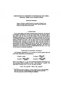
evaluation. 4 The performance of our implementation is reasonable but not perfect: for 150 3-quadric configurations involving 650 intersections, 663 intersections are found; among them, 13 intersections are bogus and 29 intersections are not accurate enough (one or more coordinates of an intersection has less than 6 correct digits). Thus over 90 percent of the values computed by the algorithm were correct to better than 6 digits. This outcome is rather satisfactory given that determinant expansions and GCD computations have to be performed using floating-point arithmetic with limited precision. A detailed description of the experiment and an analysis of our results follow. 5.1 Empirical Results The typical situations under which purely algebraic methods for curve and surface intersections have been known to fail in practice involve various types of degeneracies such as tangencies or reducible intersections (i.e., intersection curves which are a pair of conic sections or a line plus a space cubic). Such conditions are difficult to detect and handle reliably when armed only with algebraic coefficients for the curves and surfaces. To understand how our method works in practice, we examined a number of test cases, representative examples of which are shown in Figures 1-4. In Figure 1, the cone and sphere intersect in a degenerate nodal space quartic. The cylinder intersects this quartic in four points. There are two degeneracies illustrated in Figure 2(a). The two cylinders intersect in a pair of ellipses, and the horizontal cylinder intersects the cone in a line and a space cubic. In Figure 2(b) we remove the first of these degeneracies by shrinking the size of the vertical cylinder. Then in Figure 2(c) we remove the second degeneracy by translating the horizontal cylinder down by a small amount. Figure 3 also has a degeneracy in that the two cylinders intersect in a pair of straight lines. Finally, the cone and cylinder of Figure 4 intersect in a nondegenerate space quartic with two branches, and the sphere intersects both the cone and the cylinder in nondegenerate one-branch space quartics. Correct results were generated for these and all other cases we tried. The points of intersection computed by our algorithm are illustrated in the figures by white M’s. The intersection curves from two of the three pairs of quadrics are also shown in yellow and cyan, respectively. We wanted to understand how sensitive the calculations were to small perturbations in the coeftlcients. Furthermore, this method introduces a certain coordinate axis bias since it tries to find roots along one axis at a time. Our approach to understanding the sensitivity while minimizing the effects of coordinate axis bias is given below. In the following we speak of geometric versus algebraic descriptions. The former representation is baaed on storing, for example, a center point and radius for a sphere. The latter is
41n our evaluation only natural quadrics are used, since another intersection algorithm is needed to verify the results. This should not be construed to mean that the algorithm works only for natural quadrics. ACM Transactions
on Graphics,
Vol.
10, No. 4, October
1991.
Using Multivariate Resultants to Find the Intersection
393
Figure 1
based on storing the 10 coeffkients of the general second degree equation in X, y, and z. See Miller [121 for details. For each of the cases illustrated in Figures l-4, a series of tests were performed. The ith test did the following: 1. Copy the original geometric data describing the quadrics to Qr, Qs, and Q3. 2. Generate the algebraic representations from the geometric ones, and intersect the 3 quadrics using the algorithm described in this paper. Save the results. 3. Generate i random rotation axes and i random angles in the range - T to + K. Save the axes and angles. 4. forj= lto ido Qk = rotation j applied to Qk, k = 1 to 3. 5. Generate the algebraic representations from the (transformed) geometric ones and intersect the 3 quadrics using the algorithm described in this paper. Save the results. 6. for j = i downto 1 do Qk = inverse of rotation j applied to Qk, k = 1 to 3 7. Generate the algebraic representations from the (transformed) geometric ones and intersect the 3 quadrics using the algorithm described in this paper. Save the results.
Note that we perform all basic modeling and editing on the geometric representation, and we only convert to the algebraic form when we are ready to apply the algorithm of this paper. That is why the test procedure applied ACM Transactions on Graphics, Vol. 10. No. 4, October 1991.
394
l
E.-W. Chionh et al.
(4
Figure 2 ACM Transactions on Graphics, Vol. 10, No. 4, October 1991.
Using Multivariate Resultants to Find the Intersection
395
Fig. 2. (Continued)
the rotations to the geometric representations instead of to the algebraic ones. We believe this approach is reasonable since it exactly mirrors the overall modeling environment in which such an algorithm would exist. Experience has shown that database representations and modeling operations based on geometric descriptions are far more robust than ones built on algebraic representations 171. For the ith test at steps 2, 5, and 7, there were never any errors at steps 2 or 7; the results at step 5, however, were occasionally incorrect. There were no missing intersections. Nevertheless two types of errors did occur when potential intersections were computed but deemed not to lie on the quadric surfaces when substituted back into the implicit equations: these intersections were either bogus or insufficiently accurate. The number of times these errors occurred at step 5 for the given test cases is summarized in Table I. As expected, the situations involving degeneracies generally fared the worst. 5.2 Analysis of the Empirical Results
A major concern in our implementation is the use of floating-point GCD computations, which are known to be highly instable. In our implementation, there are two occasions where GCD computations are needed: removing extraneous factors from the multivariate resultant R, (or R,, R,) and solving three equations in two variables; that is, after one of the variables x, y, z is calculated, we need to solve for the other two variables using the original three quadric surface equations. The GCD computations for ACM Transactions on Graphics, Vol. 10. No. 4, October 1991
396
-
E.-W. Chionh et al
Figure 3
Figure 4
ACM Transactions on Graphics, Vol. 10, No. 4, October 1991
Using Multivariate Resultants to Find the Intersection Table I.
1
Degeneracies Nodal
Fig. 2(a)
of Errors
space
2 ellipses
Total
quartic
and line + space
Inaccurate
Bogus
Total errors
100
0
0
0
150
13
3
16
Fig. 2(b)
Line
150
11
5
16
None
100
4
4
8
Fig,
2 lines
100
0
0
0
50
1
1
2
Fig, 4 Note.
cubic
of intersections
Fig. 2(c) 3
+ space
cubic
397
at Step 5
Number
Figure number Fig.
Summary
.
None There
are no errors
at Steps
2 and 7,
extraneous factors can be done with a high degree of accuracy, since the two polynomials involved are arrived at with very little computation (see (25), (26), and (27)). Furthermore, in practice, there may not be any extraneous roots— for example, when the rank of matrix (8) is 3. The same cannot be said for the GCD computations involved in solving three equations of two variables. The roots obtained from the intersection polynomial certainly do not have the same degree of accuracy as the coefficients of the quadric equations since the intersection polynomial is obtained after some determinant expansion; consequently the coefficients of the three quadric equations in the two remaining variables are not as accurate as the given quadric surface coeffi cients. But GCD computations in this context do not require as much accuracy, for we know that the GCD has to be a nonconstant polynomial; that is, we only need to identify nearby roots of two polynomials. Thus our algorithm finds all the intersection points, at the price of admitting some bogus intersections of coordinates that are not sufficiently accurate (in our experiments this means less than 6-digit accuracy). Bogus intersections can easily be detected; they are simply too far from one or more of the quadrics. Intersections with inaccurate coordinates can easily be polished with Newton –Raphson iteration. In our implementation, we simply applied Newton- Raphson to any point in error (that is, bogus or inaccurate), The bogus roots converged to actual intersection points, and the inaccurate points were refined. This refining procedure is qualitatively different from using Newton- Raphson for equation solving. An average of two or three iterations were sufficient to refine an inaccurate root to an acceptable value. This treatment of bogus roots required a final filtering operation to make sure that roots were not recorded multiple times, but allowed us to avoid having to distinguish between inaccurate and bogus roots. Supplemented by this Newton-Raphson refinement, then, the method has yet to fail in any of our experiments. 6. CONCLUSION To best address the practicality of the techniques described in this paper, we must again consider the larger context in which they are to be applied. In particular, recall step 1 of the Boundary Evaluation algorithm described in Section 1. We first compute the unbounded intersection curves between the ACM Transactions
on Graphics,
Vol. 10, No. 4, October
1991.
398
E.-W,
●
Chionh et al.
unbounded quadric surfaces on the model. These curves are then partitioned into pieces such that the interior points on each piece will have an identical classification surfaces
(INSIDE,
on the
A robust quadrics
implementation is as follows.
curves
using
the
[181, detecting cases
in
schemes tioned
the
addressed
the
implicit
polynomial curves
condition
ON)
with
by
isolated
When
respect
Certainly
Miller
[121.
substituting
the
representation in the
curve
between which
will
of the
The
to
all
of
3
have
Miller
[131,
the
these
other
quadric
of the
natural
straight
line
are
detected
surface
O’Connor
curves, lines
Only
context
points,
straight
quadric
quadrics been
in the quadric
intersection
parametric
parameter.
the
at least
underlying
partitioning
possible.
fashion
works the
methods
sections,
process.
in this
which Compute
geometric
conic
whenever
be
tion
OUTSIDE,
model.
use
plus
[17],
and
and
when
solving all
other
robust
conies space
representation and
intersection
the
resulting pairwise
geometrically
quartic “by
be parti-
cubic of the
Piegl
geometric
can
of the
nondegenerate
or
reducible
case cubic
can into
degree
6
interseccurves
default”
(a since
of the previous cases will have been discovered) are the algebraic schemes of this paper invoked. Our experience indicates that the application of these methods in that framework is highly reliable. The techniques described in this paper (as well as the other conic curve and quadric surface intersection schemes surveyed in the introduction) are applicable in any modeling system which has conies and quadrics as one of its geometric forms. As with any nontrivial software application, the architecture of modeling systems ought to be layered so that high-level modules are unaware of the actual curve and surface representations. When such a high-level module requires the intersection of two geometric entities, it ought simply to call a low-level intersection utility that examines the types of the two objects and invokes an appropriate intersection algorithm. If, for example, this low-level routine receives two natural quadrics, then the relevant quadric-quadric intersection algorithm can be invoked. If it receives a quadric and a rational B-spline, then it might need to convert the quadric to a rational B-spline and invoke the routine that intersects two rational B-splines. This architectural philosophy is especially important for the robust practical implementation of the technique described in this paper. Suppose (e.g., during the course of the Boundary Evaluation algorithm) that a nondegenerate 4th-degree quadric surface intersection curve (c) is generated from the intersection of quadrics Q 1 and Q2. Suppose further that it must now be partitioned at its points of intersection with another quadric surface (Q3). The algorithm of choice depends upon the types and relative geometric orientations of the three quadrics. For example, it may be the case that Q1 intersects Q3 in a degenerate curve of some sort. If so, it will be more reliable numerically to compute these degenerate intersection curves and then intersect them with Q2 than it would be to do a 3-quadric intersection. On the other hand, if there are no degeneracies between any of the 3 quadrics, then the methods of this paper are numerically reliable and ought to be used. There is another aspect to this claim of “broader than quadrics” applicability. The method of multivariate resultants can, in theory, be applied to none
ACM Transactions
on Graphics,
Vol.
10, No. 4, October
1991.
Using Multivariate Resultants to Find the Intersection
higher order surfaces. reasons:
We chose to study quadric
(1) to test the method on the simplest nonplanar (2) the resultant matrices get intractably the surface degree rises; (3) there are some nice quadric-specific denominators (cf. Section 3).
intersections
.
399
for several
case;
large (given today’s technology) tricks that allow us to eliminate
as the
The only real obstruction with respect to using these techniques with higher order surfaces is the size of the matrices involved. As computers get larger and faster, this will become less of a problem. Now that the theory has been developed and tested in the realm of quadrics, we should be able to use it for higher order surfaces when the requisite computer hardware technology reaches a suitable level. The practical applicability of this approach has been established. It provides a solution when nonnatural quadrics are involved; for natural quadrics, it provides a plausible alternative to existing algorithms.
ACKNOWLEDGMENTS
We would like to thank John Canny of the University ley, for informing us of Macaulay [9].
of California,
Berke-
REFERENCES 1. BAJAJ, C., GARRITY, T., AND WARREN, J. On the applications of multi-equational resultants, Tech. Rep. CSD-TR-826, CAPO Rep. CER-88-39, Computer %ience Department, Purdue University, West Lafayette, Ind., Nov. 1988. 2. CANNY, J. The Complexity of Robot Motion Planning. M.I.T. Press, Cambridge, Mass., 1988. 3. CHAR, B. W., GEDDES, K, 0., GONFJET,G. H., AND WATT, S. M. WATCOM Publications Ltd., 1985. 4. CHXONH,E. W. Base points, resultants, and the implicit representation Ph. D. dissertation,
University
of Waterloo,
Waterloo,
Ont.,
Canada,
Maple User’s Guide. of rational
surfaces
1990.
5. COLLINS, G. E.
The calculation of multivariate polynomial resultants. J. ACM 18, 4 (Oct. 1971), 515-522. 6, FAROUKI, R. T., NEFF, C. A., AND O’CONNOR, M. A. Automatic parsing of degenerate quadric-surface intersections. ACM Trans. Graph. 8, 3 (July 1989), 174-203. 7. GOLDMAN,R. N. Two approaches to a computer model for quadric surfaces. IEEE Cornput. Graph. Applicatwns 3, 6 (Sept. 1983), 21-24.
8. LEVIN, J. Mathematical models for determining the intersections of quadric surfaces. Comput. Graph. Image Process. 11, 1 (Sept. 1979), 73-87. 9. MACAULAY, F. S. Note on the resultant of a number of polynomials of the same degree. Proc. London Math. Sot. (June 1921), 14-21. 10. MACAULAY, F, S. On some formula in elimination. Proc. London Math. Sot. (May 1902), 3-27. 11. MACAULAY, F. S. The Algebraic Theory of Modular Systems, Stechert-Hafner Service Agency, New York, 1964. 12. MD,LER, J. R. Analysis of quadric surface based soIid models. IEEE Cornput. Graph. AppL 8, 1 (Jan. 1988), 28-42. 13. MILLER, J. R. Geometric approaches to nonplanar quadric surface intersection curves. ACM Trans. Graph. 6, 4 (Oct. 1987), 274-307. ACM Transactions on Graphics,
Vol. 10, No. 4, October
1991.
400
.
E.-W. Chionh et al.
14, MORGAN, A. P., AND SARRAGA, R. F. A Method For Computing Three Surface Intersectwn Points in GMSOLZD. Research Publication GMR-3964, General Motors Research Lab. 1982. 15. MORRIS, J. L. Computatwnal Methods in Elementary Numerical Analysis. Wiley, New York, 1983. 16. OCKEN, S., SCHWARTZ, J. T., AND SHARIR, M. precise implementation of cad primitives using rational parameterizations of standard surfaces. In Solid Modeling by Computers: From Theory to Applications, M. S. Pickett and J, W. J30yse, Eds., Plenum Press, New York, 1984. 17. O’CONNOR, M. A. Natural quadrics: Projections and intersections. IBM J. Res. Deu. 33, 4 (July 1989), 417-446. 18. PIEGL, L. Geometric method of interacting natural quadrics represented in trimmed surface form. Comput. Aided Des. 21,4 (May 1989). 19. REQUICHA,A. A. G., ANDVOELCKER,H. B, Boolean operations in solid modeling: Boundary evaluation and merging algorithms. Proc. IEEE 73, 1 (Jan, 1985), 30-44. 20. SALMON,G. Lessons Introductory to the Modern Higher Algebra. G. E. Stechert, New York, 1924. 21. SARRAGA, R. F. Algebraic methods for intersections of quadric surfaces in GMSOLID. Comput. Viswn, Graph. Image Process. 22, 2 (May 1983), 222-238. 22. VAN DERWAERDEN, B. L. Modern Algebra, 2nd ed,, Frederick Ungar, New York, 1950. Received July 1988; revised May 1990; accepted January Editor: Greg Nielson
ACM Transactions
on Graphics,
Vol. 10, No. 4, October
1991
1991