Using New Mode Choice Model Nesting Structures to Address ... - MDPI

sustainability Article

Using New Mode Choice Model Nesting Structures to Address Emerging Policy Questions: A Case Study of the Pittsburgh Central Business District Zulqarnain H. Khattak 1, *,† and Michael D. Fontaine 3,† 1 2 3

* †

ID

, Mark J. Magalotti 2,† , John S. Miller 3,†

Center for Transportation Studies, Department of Civil and Environmental Engineering, Thornton Hall D101, 351 McCormick Road, University of Virginia, Charlottesville, VA 22904, USA Center for Sustainable Transportation Infrastructure, 706 Benedum Hall, University of Pittsburgh, Pittsburgh, PA 15213, USA; [email protected] Virginia Transportation Research Council, 530 Edgemont Rd., Charlottesville, VA 22903, USA; [email protected] (J.S.M.); [email protected] (M.D.F.) Correspondence: [email protected]; Tel.: +1-412-608-9346 All authors contributed substantially to the research article.

Received: 19 October 2017; Accepted: 13 November 2017; Published: 17 November 2017

Abstract: As transportation activities affect a region’s environmental quality, knowing why individuals prefer certain modes can help a region make judicious transportation investments. Using a nested logit model, this paper studies the behavior of commuters to downtown Pittsburgh who use auto, bus, light rail, walking, and biking. Although statistical measures influence the selection of a nesting structure, another criterion for model selection is the policy questions such models inform. Hence this paper demonstrates how an alternative model structure allows planners to consider new policy questions. For example, how might a change in parking fee affect greenhouse gas emission (GHGs)? The proposed model showed that a 5%, 10% and 15% increase in parking cost reduces GHGs by 7.3%, 9% and 13.2%, respectively, through increasing carpoolers’ mode share. Because the proposed model forecasts mode choices of certain groups of travelers with higher accuracy (compared to an older model that did not consider the model selection criteria presented here), the proposed model strengthens policymakers’ ability to consider environmental impacts of interest to the region (in this case, GHGs). The paper does not suggest that one nesting structure is always preferable; rather the nesting structure must be chosen with the policy considerations in mind. Keywords: nested logit model; multinomial logit model; transport policy; travel behavior; econometrics; utility function; systematic term; random term; discrete mode choice; carpool; sustainable transport

1. Introduction Although one may view a city as a geographical unit, a city itself is a “functional region” defined by a series of networks—trade, communications, and transportation [1]. Not only is the environmental health of the region influenced by actions taken [2], but the very definition of what constitutes a region rests in part on the connectedness of the transportation network. Recognizing that transportation impacts both the natural world (e.g., air, noise, and water quality) and the human environment (e.g., community cohesion, economic development, and property values) [3], it is appropriate to evaluate these impacts when considering potential changes to the transportation system. For example, in the U.S. alone, $4 trillion were forecast to be spent to accommodate new commercial and residential development over a quarter century—but more than a $400 billion reduction in these

Sustainability 2017, 9, 2120; doi:10.3390/su9112120

www.mdpi.com/journal/sustainability

Sustainability 2017, 9, 2120

2 of 16

costs could be achieved with more compact development, which certain modes of transportation support [4]. Failure to consider indirect impacts of transport investments, such as additional land consumption [1], increased barriers for social interaction [3] or vehicle emissions means that a large contributor to a community’s health is ignored. Because these effects may not be easily apparent prior to investment decisions, transportation “models” may be used to help forecast demand over medium to longer periods of time (e.g., 5 to 20 years) and through considering external forces (such as changes in a region’s employment), shorter term factors (e.g., fuel costs), and longer-term initiatives (e.g., increasing transit capacity) [5]. Although a model may take many forms, it is at its essence “a series of mathematical equations that are used to represent how people travel” [6]; in a model, the impacts of a variety of decisions (do nothing at location x, build a new freight hub at location y, and expand the hours of service for transit line z) can be examined before such decisions are implemented. A model’s scope is not limited to actions dictated from a central authority; in fact, the fragmented decision-making structure of U.S.-based metropolitan planning [2] renders it naïve to assume such an authority can implement policies with no other institutional support. Gossling [7] and Feng [8] differentiate between such investments that entail a directive (also described as “command and control”; examples are law enforcement moving crowds after a sporting event or speed limits) and two other actions that do not require a centralized entity. These are: (1) investments that provide information only (e.g., changeable message signs indicating travel times on parallel routes thereby enabling travelers to reduce delay if they so choose); and (2) market-based approaches that are a combination of the former two categories (e.g., taxes on certain routes and subsidies for certain modes of travel). The role of the model is thus to provide information to decision-makers regarding the costs and benefits of potential investments, and this role can be served in a variety of planning contexts. For example, the model developed herein shows how work trips (relative to other trip purposes) tend to increase bus use more than they increase light rail use. While such a finding could, in limited situations, inform a command-and-control measure (such as the provision of bus-only lanes during peak periods), its relevance is more apt for “soft” policies [7] such as apps allowing travelers to compare this mode to the cost of other modes or market-based policies (e.g., a change in fares during peak periods). 2. The Niche for Discrete Mode Choice Models Metropolitan residents have the option to choose from different travel modes multiple times throughout the day. Since the cumulative effect of these decisions affects the environment, understanding how travelers choose among these alternatives matters for policymakers. Some factors are specific to a given mode (e.g., travel time, cost, comfort, and reliability); others are specific to the traveler (income, awareness of alternatives, and the reason for the trip). As mode choice is a complex decision making process for each person, a large sample of individual choices are used to extract insights despite seemingly random variation [9]. For example, slower modes might be tolerated to a greater degree by commuters with less disposable income than by wealthier travelers. Because an individual’s socioeconomic characteristics are a critical part of the decision process, and because some of these data can only be obtained through relatively expensive survey methods, transportation agencies have a vested interest in being able to mine historical survey-based data sets, such as travel diaries. However, new policy questions are emerging with the passage of time that may not have been emphasized just a few years ago when diaries were collected. Hence, there is a need to better understand how alternative model structures can be applied to answer such questions. This paper addresses that need by demonstrating how an alternative discrete choice model structure can answer one such question: how do changes in age and parking cost influence willingness to carpool? While carpooling itself is an old mode, the advent of a new supplier—the transportation network company (TNC)—has increased opportunities to share a vehicle and thus generated new interest in the factors that influence ridesharing. While some of this benefit results from improved

Sustainability 2017, 9, 2120

3 of 16

model accuracy, the need to develop a model to address a specific question—rather than presuming one model can answer all questions—is germane. The paper thus has three objectives:

• • •

To determine if altering the nesting structure affects the ability of discrete choice models to address questions of interest. To demonstrate the impact of such a revised structure on forecast accuracy. To quantify how better models, influence estimation of environmental impacts (e.g., how increased vehicle sharing may affect emissions).

The first bullet is significant because new nesting structures can incorporate new variables, and there is an increased understanding that the individual socioeconomic characteristics influence mode choice as much as transportation characteristics [10–12]. The second bullet is of interest because while much literature [13–16] has focused on modeling decisions, less frequently have models been validated for transferability to similar regions [2,17,18]. (This paper assesses the model’s accuracy using a different data set than that used to build the model, thereby helping to provide guidance on transferability elsewhere.) The third bullet is important because impacts on greenhouse gas emissions (GHGs) are increasingly considered in transport investment decisions [19,20]. Thus, assessment of how changes in certain mode shares, such as carpooling, affects GHGs is an integral component of future policy decisions. While the paper uses a data set for an urbanized section of Pittsburgh, Pennsylvania as a case study, the demonstration of the value of new modeling structures for answering new questions is relevant to other municipal locations seeking to maximize the benefit of existing discrete choice data sets. An extensive amount of literature related to mode choice decisions provides a starting point for considering model refinements [10]. Less attention has been paid to forecast accuracy and using revised model structures to address policy questions of interest.

•

•

•

Following the advocacy of econometric techniques for discrete choice modeling, some studies employed explicit modeling of latent psychological explanatory variables, heterogeneity, and latent [9,21]. Others have integrated two decisions via a combined mode and departure time choice model [22,23]. Two other studies [24,25] used multinomial logit models to study intercity travel behavior in Libya and choice behavior of concert participants at Taipei Arena, respectively. Wang et al. [26] developed binary and nested logit models to check the extent to which visitors’ individual attributes (e.g., income, travel frequency distance, and home delivery) influence shopping trip mode choices. Subbarao [27] developed a typology of trip chains based on the structure and activity of trips in a metropolitan region of India, and later proposed a nested logit model. Another study [28] used integrated choice and a latent variable model to examine the factors influencing school teenagers’ travel decisions. Gao et al. [29] reviewed how altering public transit networks can improve the performance of mode choice forecasting. Two recent studies [30,31] considered commuters’ willingness to carpool using cross nested model structures. Discrete choice models are not limited to mode selection but include highway safety [32], express delivery service [33], travelers’ willingness to pay for better quality information [34], and economic impacts of disruptions to entire industries [35]. Forecast accuracy, especially the desire to make models transferable, has been a motivation for discrete choice models in particular [14]; Rossi and Bhat [36] summarize related efforts. Tellingly, however, the authors state that “There is no basis in the research for defining situations in which model parameters are clearly and definitively spatially transferable [36].” For the study’s third objective, some authors have developed models for policy questions of interest to non-modelers. Schlaich [37] showed that logit modeling can inform investments made in traveler information; at one location, variable message signs led to a maximum diversion rate of 30%. Kalaee et al. [13] showed that students not in neighborhood schools, students from families with high income, high school students, and female students are less likely to walk or

Sustainability 2017, 9, 2120

4 of 16

bike in comparison to other students. Veras and Wang [38] concluded that time factors instead of cost factors are more influential in choosing an electronic toll collection system. Islam et al. [15] showed how mode choice behavior of park and ride users was affected by transit vehicles and transfer time at stations using logit models. A hypothetical hurricane scenario presented to Miami residents-showed that although special evacuation buses were the most likely mode choice, other modes could be favored such as taxi (wealthy evacuees) or regular bus (evacuees destined for a hotel) [14]. Incentives for carpooling (e.g., [39–41]) have also received attention; this paper however, contributes to these existing studies by seeking to explicitly consider the carpooling and vanpooling to16an existing Sustainability 2017,modes 9, 2120 as discrete alternatives and comparing the proposed model4 of model used in practice for forecast accuracy and validation in order to provide guidance on this paper however, contributes to these existing studies by seeking to explicitly consider the transferability to other regions.

3.

carpooling and vanpooling modes as discrete alternatives and comparing the proposed model to an existing model used in practice for forecast accuracy and validation in order to provide Motivationguidance for Considering an Alternative Nesting Structure on transferability to other regions.

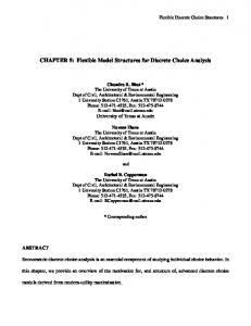
The 3. Southwestern Pennsylvania Commission is the regional planning agency serving the Motivation for Considering an Alternative Nesting Structure Pittsburgh 10-county area [42]. Figure 1 shows the travel demand model developed for the region The Southwestern Pennsylvania Commission is the regional planning agency serving the in 1989, and the structure informed certain policy questions that faced decision makers at that time. Pittsburgh 10-county area [42]. Figure 1 shows the travel demand model developed for the region in For example, model differentiates between to transit and driving tothat transit. This enables 1989,the and the structure informed certain policy walking questions that faced decision makers at time. For example,how the model differentiates between walking facilities to transit and driving to transit. This enables oneOne might one to evaluate improvements to pedestrian might influence transit use. to evaluate improvements to pedestrian might influence transit use. Oneatmight compare the cost ofhow such improvements to, say,facilities the provision of better parking such facilities, compare the cost of such improvements to, say, the provision of better parking at such facilities, and and thereby determine which initiative can increase transit patronage in the most cost-effective manner. thereby determine which initiative can increase transit patronage in the most cost-effective manner. The 2010 The survey by the Pittsburgh Partnership [43] was later used by the 2010 conducted survey conducted by the Pittsburgh Downtown Downtown Partnership [43] was later used by the Southwestern Pennsylvania Commission update some of their model,model, howeverhowever the model the model Southwestern Pennsylvania Commission totoupdate somefeatures features of their was not recalibrated andstructure the structure was alsoleft left intact. was not recalibrated and the was also intact.

Figure 1. Original Mode Choice Model Developed for Pittsburgh. Figure 1. Original Mode Choice Model Developed for Pittsburgh.

the passage of time since development ofofthe original model structure, new information With the With passage of time since thethe development the original model structure, new information has become available that suggests it may be productive to revise the model structure: has become available that suggests it may be productive to revise the model structure: A primary reason is that new policy questions are emerging. One question concerns A primary reason is that new policy questions are emerging. One question concerns transportation transportation network companies (TNCs), also known as “technology-enabled mobility service network companies (TNCs), also knowntransport as “technology-enabled mobility service companies,” companies,” which provide on-demand services or ride hailing [44]. As the availability of TNCs on-demand increases, a better understanding of the that cause individuals carpool generally may increases, which provide transport services orfactors ride hailing [44]. As thetoavailability of TNCs shed insight into the market for TNCs. related set of questions is whether commuter a better understanding of potential the factors that causeAindividuals to carpool generally mayvans shed insight are similar to carpools, are they a competitor to transit services (e.g., [45]), or are they complementary into the potential market for TNCs. A related set of questions is whether commuter vans are similar to such services (e.g., [46]). Another question is to what extent may carpooling be affected, if any, by to carpools, are they competitor to In transit services (e.g., [45]), are they complementary to such an increase in a driverless vehicles. fact, TNCs have started testing or such vehicles in the case study area [46]). and elsewhere For is these types extent of questions, a focus on two modes “carpool” andan increase services (e.g., Another[47,48]. question to what may carpooling be affected, if any, by “vanpool” is of interest. contrast, because it focused on whether certain managed in driverless vehicles. In fact,ByTNCs have started testing such vehicles in the lanes case should study area and allow only vehicles with at least two, three or four people in them, it was logical for the original model to differentiate among the carpool modes (e.g., two, three, or more than four occupants)—and to

Sustainability 2017, 9, 2120

5 of 16

elsewhere [47,48]. For these types of questions, a focus on two modes “carpool” and “vanpool” is of interest. By contrast, because it focused on whether certain managed lanes should allow only vehicles with at least two, three or four people in them, it was logical for the original model to differentiate among the carpool modes (e.g., two, three, or more than four occupants)—and to avoid a separate vanpool mode entirely. A related policy item is that what’s the role of environmental assessments in transportation investments; while this paper considers how GHGs may be affected by use of shared vehicles, decisions such as increased parking rates (to alter mode selection) or rezoning (to alter land development) also affect emissions [49]. Sustainability 2017, 9, 2120 5 of 16 A second reason for revising the structure is to increase model transferability. To some degree, avoidchanges a separate vanpool mode entirely. A related policy the item isnumber that what’sof thepersons role of environmental demographic affect forecasts. For example, age 65 and over is assessments in transportation investments; while this paper considers how GHGs may be affected by forecasted to increase by 78% in the U.S. between 2014 and 2040 [50]. Accordingly, the se socioeconomic use of shared vehicles, decisions such as increased parking rates (to alter mode selection) or rezoning variables (such as age, gender, and income) capture individual preference. (Adeel et al. [12] found that (to alter land development) also affect emissions [49]. females are more likelyreason thanfor males to use personal auto due model to comfort, EastonToand Ferrari A second revising the structure is to increase transferability. some degree,[11] found demographic changes affectto forecasts. For example, the number of persons age 65 and over that boys more than girls prefer walk or cycle to school, Kalaee et al. [13] found that ispreference forecasted to increase by 78% Neglecting in the U.S. between 2014 and 2040 [50]. Accordingly, theseand hence for car travel is affected by income.) these factors hampers forecast accuracy, socioeconomic variables (such as age, gender, and income) capture individual preference. (Adeel et transferability. Of particular interest to this paper, a separate validation data set [18] is fundamental to al. [12] found that females are more likely than males to use personal auto due to comfort, Easton and model development. Ferrari [11] found that boys more than girls prefer to walk or cycle to school, Kalaee et al. [13] found that preference for car travel is affected by income.) Neglecting these factors hampers forecast

4. Data Description accuracy, and hence transferability. Of particular interest to this paper, a separate validation data set [18] is fundamental to model development.

This study used a stated preference survey designed by the Pittsburgh Downtown Partnership [43] Data Description in 2009 and4. conducted in 2010. The emphasis of the survey was the transportation needs of Pittsburgh regional residents who worked in downtown. Data from the survey concerning factors that influence This study used a stated preference survey designed by the Pittsburgh Downtown Partnership [43] in 2009 and conducted in 2010. The emphasis of the survey was the transportation needs of 1989 [51]. travel decisions were used to update some features of the original model developed in Pittsburgh regional residents who worked in downtown. Data from the survey concerning factors The survey was released to each employer’s human resources manager and was made available to that influence travel decisions were used to update some features of the original model developed in individual1989 workers in survey that company. The was distributed to residents emails [51]. The was released to survey each employer’s human resources manager using and was made and hard copies. The workers and residents with a response time ofto one month in order to available to individual workers were in thatprovided company. The survey was distributed residents using emails and hard copies. Thenine workers and residents weredowntown provided witharea a response of oneto month receive most responses. In total, districts near the were time selected participate in in order to receive most responses. In total, nine districts near the downtown area were selected to the survey, as shown in Figure 2. participate in the survey, as shown in Figure 2.

Figure 2. Map of Nine Districts included in the Downtown Pittsburgh Survey (Source: Pittsburgh

Figure 2. Map of Nine Districts included in the Downtown Pittsburgh Survey (Source: Pittsburgh Downtown Partnership Survey, base map © Google Earth [52]). Downtown Partnership Survey, base map © Google Earth [52]).

Sustainability 2017, 9, 2120

6 of 16

A total of 6513 surveys were completed during the survey period. The survey data included information on demographic and socioeconomic characteristics, travel purpose, commute distance, parking fee, and many other factors that might influence mode choice such as travel cost, travel Sustainability 2017, 9, 2120 6 of 16 time, number of workers in the household, and vehicle ownership. Respondents were asked to select total of of 6513 surveys were completed during the survey period.biking, The survey data included between seven Amodes transport (bus, light rail transit, car, walk, carpool, and vanpool) information on demographic and socioeconomic characteristics, travel purpose, commute distance, based on various factors affecting their travel decisions. The descriptive statistics for the explanatory parking fee, and many other factors that might influence mode choice such as travel cost, travel time, variables used to generate the model are provided in Table 1. number of workers in the household, and vehicle ownership. Respondents were asked to select between seven modes of transport (bus, light rail transit, car, walk, biking, carpool, and vanpool) Table 1. Descriptive statistics of explanatory Variables. based on various factors affecting their travel decisions. The descriptive statistics for the explanatory variables used to generate the model are provided in Table 1. Variable Description Mean Min Max Table 1. Descriptive statistics of explanatory Variables.

Demographic and Socioeconomic Variable Description Indicator Variable expressing Marital Status (1 if married) Demographic and Socioeconomic Indicator Variable Variable for Gender (1 ifexpressing female) Marital Status (1 if married) Household income ($K) Variable for Gender (1 if female) Variable for Raceincome (1 if Hispanic) Household ($K) Variablecharacteristics for Race (1 if Hispanic) Trip related Variable distance from downtown (miles) Tripfor related characteristics Variable for distance from (miles) Variable for Purpose of trip (1 ifdowntown work) Variable for Purpose of trip (1 if work) Variable for Travel Time (sec) Variable for Travel Time (sec) Parking related characteristics Parking related characteristics Variable for Parking cost (1 if >$30) Variable for Parking cost (1 if >$30) Household characteristics Household characteristics Number of people age 45 and Number of people age 45 over and over livingliving in theinhousehold the household

0.52

Mean 0

Min

0.62

0.52 0

0

56

2 0.62 560 0.21 0.4 13 0 0.86 300 2340

0 300

200 1 1200 1 48 48 1 1 4500 4500

0.51

0 0.51

0

11

0.43

0 0.43

0

22

0.21 13 0.86 2340

0 2 0 0.4

1Max 11

5. Methodology 5. Methodology The modeling of this discrete choice problem for travel modes involves the seven discrete

The modeling of this discrete choiceinterested problem for travel modes the seven outcomes shown in Figure 3. (Readers in modeling details shouldinvolves refer to Appendix A.) discrete outcomes shown in Figure 3. (Readers interested in modeling details should refer to Appendix A.)

Figure 3. Two-Level Nested Logit Model for Pittsburgh Traveler Mode Choice. Figure 3. Two-Level Nested Logit Model for Pittsburgh Traveler Mode Choice.

A nested logit model consisting of three final mode choice groups were public transportation modes (including modes available for general public), private transportation modes (including modes that are private property of travelers) and commuter pool modes (consisting of ridesharing options). The data for the 6513 travelers were then split into two groups: 70% of these data points (e.g., 4559)

Sustainability 2017, 9, 2120

7 of 16

were used for calibration—e.g., developing the model. The remaining 30% (e.g., 1954 data points) were used for validation and thus never used for calibration. Multiple nesting structures were considered based on three criteria. First, the authors assessed the extent to which alternative structures demonstrated a competitive relationship among alternatives (within the nest) and hence were representative of true behavior. (For example, a nest that includes walking and biking may be appealing because of the common element of active transport; however, because the lengths of such trips differ substantially, another plausible nest is one that includes both bus and biking because of the common elements of not requiring auto ownership and comparable trip lengths). Second, because many plausible nesting structures exist, the likelihood ratio test (Appendix A) was used to test the significance of selected nest over the rejected one. A third criterion was whether the inclusive value parameters are reasonable. 6. Results and Discussion 6.1. Best Model Table 2 shows the best model based on calibration from 70% of the data. For example, after evaluating multiple models, the best model includes a parameter of 4.87 for using the drive-alone car mode (if married), and the t-statistic for this parameter, since it is larger than 1.96, suggests this variable is significant. The values of the McFadden pseudo R-squared and adjusted R-squared for summary statistics are greater than 0.1, suggesting that the model provides good explanatory power. Almost all of the defined variables are statistically significant. Table 2. Results for the Best Nested Logit Model. Bus

Light Rail Transit

Car

Walk

Bicycle

Carpool

Vanpool

Value (t-stat)

Value (t-stat)

Value (t-stat)

Value (t-stat)

Value (t-stat)

Value (t-stat)

Value (t-stat)

-

-

4.87 (2.76)

-

-

-

-

Variable for Gender (1 if female)

−1.243 (−3.24)

−1.187 (−2.84)

-

-

-

-

-

Variable for household income

−2.326 (−2.85)

-

-

-

-

−2.147 (−1.84)

−3.265 (−1.05)

4.163 (1.72)

3.267 (2.68)

-

-

-

-

-

Number of persons in the household age 45 and over

-

-

−5.745 (−4.32)

−3.459 (−1.73)

−4.568 (−2.87)

-

-

Variable for trip purpose (1 if work)

4.894 (3.56)

2.432 (3.24)

-

-

-

2.849 (1.68)

1.463 (1.95)

Variable for Parking cost (1 if >$30)

-

-

−6.638 (−3.45)

-

-

-

-

Travel Time

2.435 (2.45)

-

4.562 (3.67)

−5.631 (−1.89)

−4.353 (−2.86)

1.634 (3.62)

-

Variable for Race (1 if Hispanic)

1.430 (1.80)

-

-

-

-

-

-

Variable

Alternative Specific Constant Variable expressing Marital Status (1 if married)

Variable for distance from downtown

2.4 (1.8)

Goodness of Fit measures Log likelihood LL(0) Log likelihood at convergence LL(β) McFadden’s pseudo R-squared Adjusted pseudo R-squared Number of observations Inclusive Value parameter Public nest Inclusive Value parameter Private nest Inclusive Value parameter Commuter Pool nest

−4604.56 −3160.34 0.313 0.308 2370 0.76 0.84 0.23

Sustainability 2017, 9, 2120

8 of 16

All three inclusive value parameters (θm in Appendix A) are below 1.0, justifying that the three nests are appropriate and indicating that the modes possess some degree of unobserved shared effects. The lowest value of 0.23 for commuter pool, for example, suggests that carpool and vanpool are substitutable for each other and the nesting structure has taken care of the unobserved shared effects that existed between the two modes. (The literature supports at least two different ways of viewing vanpools: as similar to “larger capacity transportation modes” such as buses [53] or as similar to carpools (e.g., [54]) analyzed carpools and vanpools together, with the common feature being their exemption from tolls). Placement of vanpool in a public transportation nest along with bus and light rail resulted in illogical inclusive parameter values, in contrast to the chosen model of Figure 3. For this particular data set, therefore, it appears appropriate to treat vanpooling as more similar to carpooling. 6.1.1. Variables with Intuitive Signs Most variables have the expected signs. Household income shows a negative coefficient for bus, carpool, and vanpool, suggesting that higher incomes lead to a greater likelihood of driving alone. Travel time is also negative for walking and bicycling in the private nest: as travel time increases, travelers are more likely to substitute a private car for these non-motorized modes. Race also shows a positive coefficient for bus; however, the practical significance of this variable is lower for present-day work since Pittsburgh has a low population of Hispanics (around 2%). Distance from downtown shows a positive coefficient for bus and light rail, suggesting that travelers living farther from the downtown are more likely to choose these modes. Large parking costs, however, reduce the likelihood of using the car, as shown by this negative coefficient. The signs in the model also can inform policy initiatives. Presently, the lack of street and garage parking during peak hours, for example, coupled with the negative coefficient for parking costs in the model, points to the use of park and ride services originating outside the Central Business District (CBD). Shared driverless vehicles could also be considered as a viable alternative in the future to eliminate the need for parking in the CBD—and thus knowing whether parking cost substantially affects mode split may help forecast the attractiveness of this alternative. (The impact of how individuals might react to an increase in parking cost is the focus of Section 7.) 6.1.2. Variables Requiring Additional Interpretation For a few variables, however, the signs were different than that provided in some literature—and the reasons for differentiation require some additional interpretation. For example, these data showed that women were more likely to use public transportation than the private auto, which directly contradicts [55]. However, given that Belwal and Belwal [55] found that female travelers preferred private cars due to a “gender disadvantage in developing countries”, it appears that such a condition does not apply to Pittsburgh. The results also showed that married travelers are more likely to use a personal car than other choices and, while Table 2 alone does not provide a definitive reason, the fact that ‘family obligations’ was the second highest reason for individuals indicating they wanted a private car (Figure 4) suggests that these travelers may have needed the vehicle to pick up children from daycare or school. The results also suggest that people over the age of 45 are less likely to use active modes of transportation. The finding however, matches that of Schoner and Lindsey [56] who found that travelers age 40–49 were about two-thirds as likely to walk or bike as persons age 20–29.

Sustainability 2017, 2017, 9, 9, 2120 2120 Sustainability Sustainability 2017, 9, 2120

99 of of 16 16 9 of 16

Choosing Private Car Choosing Private Car No one to carpool with one tounpredictable carpool with Work schedule No varies/is Work schedule varies/isavailable unpredictable Free parking to me Free parking available to me Public trans. unavailable/unreliable Public trans. unavailable/unreliable Enjoy my privacy Enjoy Downtown my privacy Need my car while Need my car while Downtown Other Other Family obligations Family obligations More convenient More convenient

2 22.7 2.7 3.2 3.2 4.2 4.2 4.6 4.6 9.7 9.7 10.6 10.614.3 14.3 0 0

10 10

20 20

30 30

40 40

48.5 48.5 50 50

60 60

Figure 4. Reasons for Choosing Private Car (n = 2997). The category “Other” includes reasons not 4. Reasons Reasons for Choosing Private Car = 2997). category “Other” includes reasons not Figure 4. for Choosing Private Car (n (n =distance 2997). The category “Other” includes reasons not cited cited above, such as work late, start early, and toThe work. cited above, such as work late,early, start early, and distance to work. above, such as work late, start and distance to work.

6.2. Travel Mode Market Share Market Share Share 6.2. Travel Mode Market Figure 5 shows that that the highest market share among the three upper level nests (e.g., , Figure 55) shows showsthat that thatthe thetransport highestmarket market share among three upper level nests (e.g., Figure highest share among thethe three upper level nests (e.g., m1 , m2,, , and belongs to that public (44.6%), while personal cars represent the single highest ,m and ) belongs toamong public transport (44.6%), while personal the single highest and belongs to public transport (44.6%), whilelevel personal cars( represent the singlerepresents highest portion of portion trips (42.5%) the seven lower choices , cars .. ).represent Carpool 6.5% 3 ) of portion of trips (42.5%) among the seven lower level choices ( , .. ). Carpool represents 6.5% of trips (42.5%) among the seven lower level choices represents 6.5% of trips followed followed by walking (4%), bicycling (1.6%),(iand vanpool (0.8%). The forecasted and observed 7 ). Carpool 1 , i2 ...i trips followed bysimilar walking (4%), bicycling (1.6%), and (0.8%). The forecasted and was observed by walking (4%), bicycling (1.6%), andfor vanpool (0.8%). The forecasted observed values revealed values revealed mode shares; example, thevanpool observed modeand shares for carpool 7.5% values revealed similar mode shares; for example, the observed mode shares for carpool was 7.5% similar mode shares; for example, the observed mode shares for carpool was 7.5% (compared to 9% (compared to 9% which was forecasted by the model). The mode splits shown in Figure 5 match those (compared to 9% which was forecasted by the model). The mode splits shown in Figure 5 match those which was that forecasted by the model). Thetransportation mode splits shown in Figure 5 match those elsewhere elsewhere offer substantial public options, although American Associationthat of elsewhere that offer substantial public transportation although American Association of offer substantial public transportation options, although options, American Association of Stateinfluence Highwaythese and State Highway and Transportation Officials (AASHTO) [57] notes regional factors State Highway and Transportation Officials (AASHTO) [57] notes regional factors influence these Transportation Officials (AASHTO) [57] notes regional factors influence these shares. shares. shares.

PREFERENCE OF VARIOUS MODES PREFERENCE OF VARIOUS MODES OF TRAVEL OF TRAVEL Walk Walk

Carpool Carpool

Vanpool Vanpool

Light rail Light rail

Bus Bus

Car Car

Mode of Travel Mode of Travel

Bicycle Bicycle

0 0

5 5

10 10

15 15

20 25 20 25 Percent Use Percent Use

30 30

35 35

40 40

45 45

Figure on the the Revised Revised Model. Model. Figure 5. 5. Market Market Share Share for for the the Seven Seven Modes Modes Based Based on Figure 5. Market Share for the Seven Modes Based on the Revised Model.

6.3. Public Transport Attractiveness Collectively, respondents indicated that the most important factors contributing to their decision to use the personal car was convenience (48.5%) and family obligations (14.3%). Only 9.7% said they needed their car while downtown and only 4.6% named privacy as a factor. Substantially different results were obtained by considering respondents who chose public transport: saving money was

Sustainability 2017, 9, 2120

10 of 16

the most common reason (48.5%), with other reasons cited less: convenience (14.3%), no car (10.6%), reduced stress (9.7%), and less pollution (4.2%). These observations have three implications for policies: first, for auto use, convenience (which may include control over departure and arrival times) is critical; second, cost has a much bigger impact for those choosing transit than those choosing the auto, and third, socioeconomic factors may play a sizeable role (given the 14.3% of persons choosing the private car cited family obligations). 7. Alternative Nesting to Consider Policy Questions of Interest A question facing decision makers is what factors may affect the decision to carpool rather than drive alone—and what are the environmental consequences of intervention to influence these factors? This question matters as the “supply” of opportunities to share a vehicle may increase in the future. Although the focus herein is parking cost and persons age 45 and over as factors that may affect the decisions to carpool, the approach may be extended to other attributes that also affect willingness to carpool: road tolling, fuel pricing, education levels, job status, household income, and car ownership [39,58]. Parking is a good example both because of its influence on urban density and because it was a primary issue of interest to decision makers in the case study location. Persons age 45 and over was used because the original model omitted this variable and, with the passage of time, it has become clearer that persons age 45 and over is projected to differ substantially by 2040. Table 3 shows how an alternative model structure can help planners consider such emergent policy questions. The original structure supported a different policy question: should the occupancy requirement for managed lanes be 2, 3, or 4? That model suggested a 10% increase in parking cost would increase carpoolers’ mode share by about 1.5%. The new structure, however, suggests the same parking fee increase would raise the carpool mode share by 6.3%. Further, a 10% increase in travelers age 45 and over (a variable not included in the original model) increases the mode share of carpoolers by 3.7%. Because the proportion of persons age 45 and over is forecast to increase from 41% to 51% by 2040 [50], such socioeconomic variables may merit attention as new policy questions arise. Table 3. Considering Alternative Nesting to Answer Policy Questions of Interest. Model Original Model

Revised Best Model

Scenario

Base Mode Share for Carpool

Scenarios Mode Share for Carpool

10% increase in age 45 and over

12% *

NA

10% increase in Parking cost

12% *

13.5% *

10% increase in age 45 and over

9.8%

13.5%

10% increase in Parking cost

9.8%

16.1%

* Sum of 2 occupant auto, 3 occupant auto, and 4 occupant auto.

The revised model structure can thus answer questions regarding the environmental impact of encouraged vehicle sharing through an increase in parking cost: how would a shift from a drive-alone vehicle to shared vehicles reduce GHGs? For this demonstration, the study further focused on the example of change in parking cost only. Given an average trip length of 11.2 miles to downtown Pittsburgh, average vehicle emissions of 8887 grams (g) of carbon dioxide per gallon, a ratio of carbon dioxide to total GHGs of 0.989, and an average of 21.6 miles/gallon [59], Table 4 shows amount of GHGs based on the 4559 total trips to the downtown area. After scaling this result to reflect annual emissions for downtown travelers (not just those sampled), decision-makers can compare this impact to potential emissions reductions from other policies such as recycling programs and better insulation for low-income housing [19].

Sustainability 2017, 9, 2120

11 of 16

Table 4. Assessment of How an Increase in Parking Prices affects Greenhouse Gas Emissions (GHG).

Scenario

Revised Model

Result

Drive Alone Baseline 5% increase in parking cost 10% increase in parking cost 15% increase in parking cost

Carpool a

Trips

1922

447

Emissions (g CO2 eq)c

8,955,225

1,041,359

Trips

1673

629

7,795,053

2,930,716

Emissions (g CO2 eq)

c

Trips

1589

734

c

7,403,670

3,419,945

Trips

1440

843

Emissions (g CO2 eq) c

6,709,430

3,987,812

Emissions (g CO2 eq)

Total Emissions g CO2 eq Revised Model b

Reduction in Emissions

9,996,585

NA

9,260,411

7.3%

9,113,642

9%

8,673,336

13.2%

a

(Trips)/2; b Shifts to other modes (bicycle, walk, and bus) are not presumed to generate emissions (e.g., while some additional persons use the bus, the increase is not large enough to require additional bus service); c Greenhouse Gas Emissions, measured as carbon dioxide equivalent grams (g CO2 eq).

Table 4 shows how models can aid in policy decisions regarding parking costs in urban areas based on the expected future consequences. Table 4 suggests that by increasing parking costs, travelers prefer shifting to shared carpools, thus reducing net GHGs. A 5% increase in parking cost suggests a reduction of 7.3%, a 10% increase in parking cost suggests 9% reduction and a 15% increase in parking cost suggests a 13.2% reduction in GHGs. These numbers provide the basis for selection of future policies on parking costs to maintain a sustainable environment in dense urban settings. 8. Model Transferability The strength of discrete choice models is that they explain variation in behavior based on a wealth of individual characteristics [60] (income, gender, urban environment), making it feasible, at least in theory, to transfer such models to other locations [2,17,18] (although some “updating” [36] of the model parameters using local data will be advantageous) [32]. By contrast a model linked to a particular set of transportation analysis zones from whence the data were calibrated will likely not be transferable as no two locations will have the same zonal configuration [2]. McFadden [60] noted discrete choice models, because they do not aggregate data by zone, preserve the “detailed associations between individual circumstances and travel choices”. Thus, Rossi and Bhat [36] indicate that the likelihood of transferability is higher for person-level models than for zone-based models. While a robust model can explain some variation in a given data set, the model’s practical value depends on whether it can be used for forecasting scenarios of interest. That is, changes in a particular mode share will ultimately translate into a set of behaviors that have short-term consequences (e.g., congestion on bicycle network) and longer-term effects (e.g., consumption of land for new development and the resultant water and sewer costs). Thus, for any model, one must ask how does it perform with a different data set not used to calibrate the model? Hence, the authors determined the accuracy of the revised model, defined as the difference between model forecasts and observations, by using the validation data set (which had never been used for calibration); this approach provides the magnitude of error [18]. For example, consider the 1,954 travelers not used to develop the revised model. Individual 1 chose to carpool. A perfect model would have forecasted the probability of carpooling as 1.0 for this individual, whereas the model forecasted carpooling with a probability of 0.749. The sum of the error terms (such as 0.251 for individual 1), divided by 1954, yielded an error of approximately 23.2% for carpooling for the revised model. Table 5 shows the error for seven modes for the original model and the revised nesting structure, where lower values indicate more accurate forecasts. Table 5 suggests the revised nesting structure has higher forecast accuracy for six modes common to both models. For instance, the error for carpoolers reduces from 29.6% (from the original model) to 23.2% (for the revised model). For other regions, this exercise suggests that a revised nesting structure can be of value as the modes of interest change:

Sustainability 2017, 9, 2120

12 of 16

for instance, if one wants to differentiate between requiring two versus requiring three persons per vehicle, the original nesting structure is preferable. However, if one wants to differentiate between two non-motorized forms of transport (bike and walk) then the revised model is preferable. Table 5 is also encouraging in that for all six modes shown, the revised nesting structure reduced the forecast error. Furthermore, regions interested in transferring the model can also use their local samples to test the forecast accuracy and then update model parameters as suggested elsewhere [2,36]. Table 5. Forecast Error for Seven Modes of Interest. Nesting Structure Original Model Revised Model with New Nesting

Statistical Measure Mean absolute deviation *, ** n |ε | MAD = ∑i=1n i

Bus

Light Rail

Car

Walk

Bicycle

Carpool

Vanpool

0.287 a

NA

0.381

0.268

NA

0.296 b

NA

0.236

0.210

0.271

0.267

0.230

0.232

0.235

* ε i = Observed Outcome − Predicted Outcome; ** n = Number o f Observations; a ( Travelers using rail and buses f or at least a section o f their trip ); b ( sum o f 2 occupant auto, 3 occupant auto, and 4 occupant auto in the original model ).

Additionally, the error from Table 5 can be combined with the mode shares of Table 3 to provide a forecast range instead of a point value—thereby conveying a more realistic understanding of any model’s limitations. Table 3 shows that a 10% increase in persons age 45 and over increases the propensity of carpoolers by 3.7%. With an error of 23.2% for this mode (Table 5) and a 95% confidence level, the forecast increase is a range of 3.2% to 4.2%. 9. Conclusions and Application to Planning Practice Using the over 6000 samples from a case study conducted in Pittsburgh, the paper reports on the development of a proposed model that incorporates, at its inception, both statistical criteria and policy questions. The proposed model targets a specific question of interest: what factors lead to the decision to carpool rather than drive alone. The model shows that a 10% rise in parking cost increases carpoolers’ mode share by 6.3%—an increase that is four times the amount forecasted by the original nesting structure. Demographics are a critical component of the revised model: a 10% increase in persons age 45 and over, adds almost 4 percentage points to carpoolers’ mode share. Returning to the paper’s second objective, the proposed model appears to increase transferability, as it reduces aggregate forecast error by six percentage points. Finally, the model shows the value of what-if analyses: a 5%, 10% and 15% increase in parking costs reduces net GHGs by 7.3%, 9% and 13.2% through shifting travelers to shared carpools. This type of scenario visioning can facilitate the incorporation of environmental impacts into investment choices. The paper’s demonstration of how changing the nesting structure affects both (1) the accuracy of the model and (2) the ability to answer certain policy questions of interest contributes to the existing literature. The authors therefore, recommend that new nesting structures should be considered along with statistical criterion during model calibration in order to tailor the model to a wide range of questions that may arise. Such joint consideration of both policy questions and statistical criteria at the same time may take some coordination between modelers and analysts. (For instance, the paper showed that the inclusion of socioeconomic variables in the model matters as much as transportation characteristics since the age distribution in the U.S. is projected in 2040 to differ substantially from what is seen today.) The paper, the refore, does not suggest that one nesting structure is always preferable; rather the nesting structure should be chosen based on the policy questions at hand. The findings do show some benefits to recalibrating relatively recent data sets for that purpose. Further, because of the importance of age, income, gender, and marital status in the Pittsburgh model, there may be a benefit to collecting additional demographic data, especially with respect to trip chaining, as resources become available.

Sustainability 2017, 9, 2120

13 of 16

Acknowledgments: The authors acknowledge the effort of Pittsburgh downtown partnership in conducting the survey. Author Contributions: All authors contributed substantially to the research article. Conflicts of Interest: The authors declare no conflict of interest.

Appendix A. Justification for the Use of the Inclusive Value Parameter as a Decision Criterion (Nested Logit Model) To understand why the inclusive value parameter was relevant to model selection, it is appropriate to consider how this parameter influences the model structure. With discrete nominal choices (such as the seven modes i1 , . . . , i7 in Figure 3), utility functions link the choice outcome to the decision process and follow the form of Equation (A1) for mode i and person n. Equation (A1) shows a systematic component βXin and a random component ε in . The systematic component contains attributes perceived by the modeler (e.g., X1 might be age and β 1 would be the parameter for age) while the random component accounts for unobserved impacts such as preferences for traveler n. Because utility is not deterministic, one can only find the probability of individual n choosing mode i. With independent and identical (IID) distribution of the random terms, the probability for such a choice is given by Equation (A2) [9]. Uin = βXin + ε in (A1) Pn (i ) =

e[ βXin ] ∑ e[ βXin ]

(A2)

When the IID assumption is violated, as is the case with the alternatives of carpooling and vanpooling where errors are highly correlated, a nested logit model is preferable as shown in Figure 3. Such models eliminate the problem of unobserved correlation by nesting different alternatives [32]. After assuming the Gumbel distribution for the random term, Equation (A3) can be derived for calculation of the two level nested logit model [9] for person n, where m refers to a choice at an upper level (e.g., selecting a particular nest) and i refers to a choice at a lower level (e.g., selecting a particular alternative within a nest). Pn (i ) = Pn (i/m) ∗ Pn (m) (A3) Equation (A3) indicates that nested logit model can be expressed as a product of two probabilities: the marginal choice probability (e.g., the probability of choosing an upper level nest such as public transport) and a conditional choice probability (e.g., the probability of choosing a bus given that the traveler will use a public transport mode). Because there may still be some correlation among the upper level nests (e.g., there may be correlation between public transport and commuter pool due to random error present within lower levels of those nests), the marginal choice probability for m = public transport, private, or commuter pool is given by Equation (A4). Pn (m) =

e(Vm+µm ) ∑m0 ε Mn e(Vm+µm )

(A4)

µm represents the product of inclusive value parameter θm and LSi,m . LSi,m is estimated from the Vi

log of sum of exponents of nested utilities under consideration i.e., ln [e θm ]. The conditional choice probability for the lower level choices (i1 , . . . , i7 ) in Figure 3 is given by Equation (A5) and the product of the two choice probabilities provides the required probability for the nested logit model. Pn (i/m) =

e(Vi)µd 0

∑i0 εInm e(Vi )µd

(A5)

In Equation (A5), µd represents the inverse of inclusive value parameter θm whose appearance implies that all the parameters of the utility are scaled by a common value [10]. Logical values for

Sustainability 2017, 9, 2120

14 of 16

θm are between 0 and 1—a fact that proved critical for later evaluating the many potential nesting structures for this data set. The actual implementation of Equations (A1)–(A5) was performed with the econometric package N-Logit 4.0. The survey results were converted into the proper format for the N-logit package, including the creation of dummy variables and skipping of missing observations to clean the data properly. Because highly correlated variables are problematic [32,61], variables with correlation above 0.85 were removed from the analysis. (In this data set, travel time and cost had a high correlation coefficient of 0.96.) Then, a multinomial logit model was tested, but due to correlation effects of certain alternatives, such as vanpool and carpool, the results were not satisfactory. As an alternative approach, multiple nested logit models were created and tested to develop the best possible model having lower Akaike Information Criteria (AIC) values. The likelihood ratio test was also used to check whether the selected model was superior to the rejected models. The results for each model were tested for their statistical significance, where t-statistics larger than 1.96 (corresponding to a p-value of 0.05 for a two-tailed test) were viewed as significant. Note that in Table 2, the log-likelihood at zero may appear relatively high (e.g., closer to zero) than expected because some individuals did not have all seven modal choices available to them. Note also that because the bus system is much larger than the light rail system (that runs in a very small portion of the city) [51], approximately four times as many travelers use bus than light rail. References 1. 2. 3. 4. 5.

6. 7. 8. 9. 10. 11. 12. 13.

14. 15.

Rediscovering Geography Committee. Rediscovering Geography: New Relevance for Science and Society; National Academies Press: Washington, DC, USA, 1997. Meyer, M.D.; Miller, E.J. Urban Transportation Planning—A Decision Oriented Approach, 2nd ed.; McGraw Hill: New York, NY, USA, 2001; ISBN 0072423323. Forkenbrock, D.J.; Weisbrod, G.E. Guidebook for Assessing the Social and Economic Effects of Transportation Projects; National Academy Press: Washington, DC, USA, 2001. Burchell, R.W.; Lowenstein, G.; Dolphin, W.R.; Galley, C.G.; Downs, A.; Seskin, S.; Still, K.G.; Moore, T. TCRP Report 74: Costs of Sprawl 2000; National Academy Press: Washington, DC, USA, 2002. Federal Highway Administration; Federal Transit Administration. The Transportation Planning Process: Briefing Book: Key Issues for Transportation Decisionmakers, Officials, and Staff ; FHWA-HEP-07-039; U.S. Department of Transportation: Washington, DC, USA, 2015. Beimborn, E.A. A Transportation Modeling Primer; Center for Urban Transportation Studies, University of Wisconsin Milwaukee: Milwaukee, MI, USA, 2006. Gossling, S. Urban transport transitions: Copenhagen, city of cyclists. J. Transp. Geogr. 2013, 33, 196–206. [CrossRef] Feng, L.; Miller-Hooks, E.; Brannigan, V. Mathematical modeling of command-and-control strategies in crowd movement. Transp. Res. Rec. J. Transp. Res. Board 2014, 2459, 47–53. [CrossRef] Ben-Akiva, M.; Lerman, S.R. Discrete Choice Analysis; MIT Press: Cambridge, MA, USA, 1985; ISBN 0262022176. Koppelman, F.S.; Bhat, C. A Self Instructing Course in Mode Choice Modeling: Multinomial and Nested Logit Models; Federal Transit Administration: Washington, DC, USA, 2006; pp. 1–249. [CrossRef] Easton, S.; Ferrari, E. Children’s travel to school-the interaction of individual, neighbourhood and school factors. Transp. Policy 2015, 44, 9–18. [CrossRef] Adeel, M.; Yeh, A.G.O.; Zhang, F. Transportation disadvantage and activity participation in the cities of Rawalpindi and Islamabad, Pakistan. Transp. Policy 2016, 47, 1–12. [CrossRef] Kalaee, M.S.; Rezaeian, M.R.; Ahadi, M.R.; Shafabakhsh, G.A. Evaluating the factors affecting student travel mode choice. In Proceedings of the 50th Annual Transportation Research Forum, Portland, OR, USA, 16–18 March 2009; pp. 340–358. Mohaimin, A.; Ukkusuri, S.V.; Murray-tuite, P.; Gladwin, H. Analysis of hurricane evacuee mode choice behavior. Transp. Res. Part C 2014, 48, 37–46. Islam, S.T.; Liu, Z.; Sarvi, M.; Zhu, T. Exploring the Mode Change Behavior of Park-and-Ride Users. Math. Probl. Eng. 2015. [CrossRef]

Sustainability 2017, 9, 2120

16.

17. 18. 19. 20. 21. 22. 23.

24. 25. 26. 27. 28.

29. 30.

31. 32. 33. 34. 35. 36. 37. 38. 39.

15 of 16

Holguín-veras, J.; Paaswell, R.; Yali, A.M. Impacts of Extreme Events on Intercity Passenger Travel Behavior: The September 11th Experience I. Introduction. In Impact of Human Response to September 11, 2001 Disasters: What Research Tell Us; Special Publication #39; Natural Hazards Research and Information Applications Information Center, University of Colorado: Boulder, CO, USA, 2003; pp. 374–404. Galbraith, R.A.; Hensher, D.A. Intra-metropolitan transferability of mode choice models. J. Transp. Econ. Policy 1982, 16, 7–29. Fountas, G.; Ch, P. A random thresholds random parameters hierarchical ordered probit analysis of highway accident injury-severities. Anal. Methods Acid. Res. 2017, 15, 1–16. [CrossRef] Bernstein, W.; Gasparetti, A.; Ingram, M.; Johnson, I.; Mooney, J.; Perez, M.; Vaidyanathan, S. Greenhouse Gas Emission Inventory; Pittsburgh Climate Initiative: Pittsburgh, PA, USA, 2006. Pa.gov Sustainability Benchmarking & Recognition. Available online: http://pittsburghpa.gov/dcp/dcpsus-benchmarking.html (accessed on 10 April 2017). Ben-Akiva, M.; McFadden, D.; Train, K.; Boersch-supan, A.; Daly, A. Hybrid Choice Models: Progress and Challenges Hybrid Choice Models: Progress and Challenges. Mark. Lett. 2002, 13, 163–175. [CrossRef] Bajwa, S.; Bekhor, S.; Kuwahara, M.; Chung, E. Discrete Choice Modeling of Combined Mode and Departure Time. Transportmetrica 2008, 4, 155–177. [CrossRef] Ding, C.; Sabyasachee, M.; Lin, Y.; Xie, B. Cross-Nested Joint Model of Travel Mode and Departure Time Choice for Urban Commuting Trips: Case Study in Maryland—Washington, DC Region. J. Urban Plan. Dev. 2015, 141. [CrossRef] Miskeen, M.B.; Alhodairi, M.A.; Rahmat, R.A. Behavior Modeling of Intercity Travel Mode Choice for Business Trips in Libya: A Binary Logit Model of Car and Airplane. J. Appl. Sci. Res. 2013, 9, 3271–3280. Chang, M.; Lu, P. A Multinomial Logit Model of Mode and Arrival Time Choices for Planned Special Events. Proc. East. Asia Soc. 2013, 10, 710–727. Wang, K.; Shi, X.; Xiao, T. Analysis on Factors Associated with Shopping Transport Mode Choice and Change: A Study in Two Cities in China—Shanghai and Shenzhen. ICCTP 2010. [CrossRef] Subbarao, S.S.V.; Krishna Rao, K.V. Trip chaining behavior in developing countries: A study of Mumbai Metropolitan Region, India. Eur. Transp. 2013, 53, 1–30. Kamargianni, M.; Dubey, S.; Polydoropoulou, A.; Bhat, C. Investigating the subjective and objective factors influencing teenagers’ school travel mode choice—An integrated choice and latent variable model. Transp. Res. Part A Policy Pract. 2015, 78, 473–488. [CrossRef] Gao, J.; Zhao, P.; Zhuge, C.; Zhang, H.; Mccormack, E.D. Impact of Transit Network Layout on Resident Mode Choice. Math. Probl. Eng. 2013, 452735. [CrossRef] Dissanayake, D.; Morikawa, T. Investigating household vehicle ownership, mode choice and trip sharing decisions using a combined revealed preference/stated preference Nested Logit model: Case study in Bangkok Metropolitan Region. J. Transp. Geogr. 2010, 18, 402–410. [CrossRef] Habib, K.M.N.; Tian, Y.; Zaman, H. Modelling commuting mode choice with explicit consideration of carpool in the choice set formation. Transportation 2011, 38, 587–604. [CrossRef] Washington, S.P.; Karlaftis, M.G.; Mannering, F.L. Statistical and Econometric Methods for Transportation Data Analysis; Taylor & Francis: Milton Park, UK, 2010; Volume 2, ISBN 9781420082869. Lian, L.; Zhang, S.; Wang, Z.; Liu, K.; Cao, L. Customers’ Mode Choice Behaviors of Express Service Based on Latent Class Analysis and Logit Model. Math. Probl. Eng. 2015. [CrossRef] Khattak, A.J.; Yim, Y.P.; Stalker, L. Willingness to pay for travel information. Transp. Res. Part C Emerg. Technol. 2003, 11, 137–159. [CrossRef] Veras, J.H.; Xu, N.; Bhatt, C. An assessment of the impacts of inspection times on the airline industry’s market share after September 11th. J. Air Transp. Manag. 2012, 23, 17–24. [CrossRef] Rossi, T.F.; Bhat, C. Guide for Travel Model Transfer; Federal Highway Administration: Washington, DC, USA, 2014. Schlaich, J. Analyzing Route Choice Behavior with Mobile Phone Trajectories. Transp. Res. Rec. J. Transp. Res. Board 2010, 2157, 78–85. [CrossRef] Holguín-Veras, J.; Wang, Q. Behavioral investigation on the factors that determine adoption of an electronic toll collection system: Freight carriers. Transp. Res. Part C Emerg. Technol. 2011, 19, 593–605. [CrossRef] Buluing, R.; Soltys, K.; Habel, C.; Lanyon, R. Driving Factors Behind Successful Carpool Formation and Use. Transp. Res. Rec. J. Transp. Res. Board 2009, 31–38. [CrossRef]

Sustainability 2017, 9, 2120

40.

41. 42. 43. 44. 45. 46.

47. 48.

49. 50. 51. 52. 53.

54. 55. 56. 57.

58. 59. 60. 61.

16 of 16

Buluing, R.; Soltys, K.; Habel, C.; Lanyon, R. Catching a Ride on the Information Super-highway: Toward an Understanding of Cyber-mediated Carpool Formation and Use. In Proceedings of the 89th Annual Meeting of Transportation Research Board, Washington, DC, USA, 10–14 January 2010. Minett, P.; Pearce, J. Estimating Energy Consumption Impact of Casual Carpooling. In Proceedings of the 89th Annual Meeting of Transportation Research Board, Washington, DC, USA, 10–14 January 2010. SPC Southwestern Pennsylvania Commision Official Website. Available online: http://www.spcregion.org/ (accessed on 17 April 2017). PDP Pittsburgh Downtown Partnership. Available online: http://www.downtownpittsburgh.com/ (accessed on 18 May 2017). Committee for Review of Innovative Urban Mobility Services Between Public and Private Mobility-Examining the Rise of Technology Enabled Transportation Services; The National Academies Press: Washington, DC, USA, 2015. Kilani, M.; de Palma, A.; Proost, S. Are users better-off with new transit lines? Transp. Res. Part A Policy Pract. 2017, 103, 95–105. [CrossRef] Gallivan, F.; Ang-Olson, J.; Liban, C.B.; Kusumoto, A. Cost-Effective Approaches to Reduce Greenhouse Gas Emissions Through Public Transportation in Los Angeles, California. Transp. Res. Rec. J. Transp. Res. Board 2011, 2217, 19–29. [CrossRef] CBS Uber Self-Driving Car Hits the Streets of Pittsburgh. Available online: http://pittsburgh.cbslocal.com/ 2016/09/14/uber-driverless-cars-hit-the-streets-of-pittsburgh/ (accessed on 5 April 2017). Blazina, E.; Moore, D. Uber Self_Driving Cars resume service in Pittsburgh and Tempe. Available online: http://www.post-gazette.com/business/tech-news/2017/03/27/Uber-driverless-cars-voluntary-suspendtesting-halted-Pittsburgh-Mayor-Bill-Peduto/stories/201703270139 (accessed on 8 July 2017). Rossen, L.M.; Pollack, K.M. Making the Connection Between Zoning and Health Disparities. Environ. Justice 2012, 5. [CrossRef] Colby, S.L.; Ortman, J. Projections of the Size and Composition of the U.S. Population: 2014 to 2060; U.S. Census Bureau: Washington, DC, USA, 2015. Baker, M. SPC Regional Travel Model Revised Mode Choice Component; Southwestern Pennsylvania Commision: Pittsburgh, PA, USA, 2015. Google Maps from Google Earth. Available online: https://www.google.com/permissions/geoguidelines/ attr-guide.html (accessed on 7 November 2017). Castrillon, F.; Roell, M.; Khoeini, S.; Guensler, R. I-85 High-Occupancy Toll Lane’s Impact on Commuter Bus and Vanpool Occupancy in Atlanta, Georgia. Transp. Res. Rec. J. Transp. Res. Board 2014, 2470, 169–177. [CrossRef] Pessaro, B.; Buddenbrock, P. Managed Lane Toll Prices: Impact of Transportation Demand Management Activities and Toll Exemptions. Transp. Res. Rec. J. Transp. Res. Board 2015, 2484, 159–164. [CrossRef] Belwal, R.; Belwal, S. Public Transportation Services in Oman: A Study of Public Perceptions. J. Public Transp. 2010, 13, 1–21. [CrossRef] Schoner, J.; Lindsey, G. Differences Between Walking and Bicycling over Time: Implications for Performance Management. Transp. Res. Rec. J. Transp. Res. Board 2015, 2519, 116–127. [CrossRef] AASHTO (American Association of State Highway and Transportation Officials). Commuting in America: The National Report on Commuting Patterns and Trends; American Association of State Highway and Transportation Officials: Washington, DC, USA, 2013. Dissanayake, D.; Morikawa, T. Household travel behavior in developing countries: Nested logit model of vehicle ownership, mode choice, and trip chaining. Transp. Res. Rec. 2002, 1805, 45–52. [CrossRef] EPA Greenhouse Gas Emissions from a Typical Passenger Vehicle. Available online: https://www.epa.gov/ greenvehicles/greenhouse-gas-emissions-typical-passenger-vehicle-0 (accessed on 7 November 2017). McFadden, D.L. The path to discrete-choice models. Access 2002, 20, 2–7. Fink, J.; Kwigizile, V.; Oh, J.S. Quantifying the impact of adaptive traffic control systems on crash frequency and severity: Evidence from Oakland County, Michigan. J. Saf. Res. 2016, 57, 1–7. [CrossRef] [PubMed] © 2017 by the authors. Licensee MDPI, Basel, Switzerland. This article is an open access article distributed under the terms and conditions of the Creative Commons Attribution (CC BY) license (http://creativecommons.org/licenses/by/4.0/).