Synthesis of High Degree Earth Geopotential Models ... geopotential models up to a degree and order of ... Some computer programs to calculate the gravity.
Using Personal Computers in Spherical Harmonic Synthesis of High Degree Earth Geopotential Models A. Bethencourt Escuela Superior de Ingenieros en Geodesia y Cartografía. Universidad Politécnica de Madrid. Campus Sur Ctra. Valencia km. 7 28034 Madrid. Spain J. Wang, C. Rizos, A. H. W. Kearsley School of Surveying & Spatial Information Systems, The University of New South Wales, Sydney NSW 2052, Australia Abstract. We have created software using Matlab™ to obtain gravimetric quantities from very high degree Earth Geopotential (EGM) models. This program computes gravitational (V), gravity (W) or disturbing (T) potentials, gravity (∆g ) or height ( ζ ) anomalies, the components of the vertical deflection ( ξ , η ) and the undulation of the geoid (N). These gravimetric quantities can be calculated at an isolate point, on an evenly spaced geographical grid (specified by the coordinates of two of its corners) with a certain resolution, or at an arbitrary array of points whose coordinates are given in a pair of vectors containing the latitudes and longitudes of these points. This program was developed using an efficient procedure that overcomes the problems of stability when using geopotential models up to a degree and order of 2700. We have compared the modified recursion techniques of Libbrecht (1985), recently reviewed and generalized by Holmes and Featherstone (2002), and the Clenshaw (1955) summation method (Tscherning and Poder, 1982). Keywords: Associated Legendre functions, Spherical Harmonics, Gravity quantities, Matlab™ Software.
1 Introduction Pavlis et al. (2004) has recently announced a new EGM complete to a degree and order 2160. With such a very high degree geopotential model it is possible to obtain the potential and related gravity quantities with a resolution never before. This new high order (short wavelength) EGM has important implications in many geodetic applications, such as the determination of the orthometric heights without levelling (via the geoid undulation and GPS measurements), or the determination of other related gravimetric quantities, e.g. the gravity
anomalies or the components of the vertical deflection. However, to obtain the gravitational potential and its related quantities from a high degree EGM is a very demanding task from the computational point of view. We need to be very careful with the following numerical aspects: (a) efficiency in the necessary time to compute the Associated Legendre Functions (ALFs) and its derivatives, the trigonometric functions, its products with ALFs and the partial sums. It strongly depends on the algorithms and also on the computer, compiler and program used; (b) accuracy; specifically in connection with the rounding-errors and their propagation that is necessarily implicated ni the arithmetic of finite precision; and (c) stability and the problems of numerical underflow and overflow. Some computer programs to calculate the gravity quantities have been published. Special mention is made of Rizos (1979), Colombo (1981), Rapp (1982) and the Tscherning/Goad (1983) programs. All of them have been reviewed in Tscherning et al. (1983). Another two more recent computer programs are described by Smith (1998) and Sanso et al. (2001). All these programs have been developed in the Fortran language. Rizos’ and Colombo’s programs compute height or gravity anomalies on an evenly spaced grid. Rapp’s program evaluates point-by-point, and for the five following gravimetric quantities: N , ∆g , ξ , η and the gravity disturbance δ g . Tscherning and Smith programs use Clenshaw’s method of summation: the first one to obtain the height and gravity anomaly and the second one to obtain the most important gravimetric (and even other related geometric) quantities. The two latter ones can perform the calculations on a point-by-point basis or on a geographical even spaced grid. The last one, the Sanso et al. program, doesn’t use Spherical Harmonic Functions but rather Ellipsoidal Harmonic, so its problems are different. All of these programs had been developed in order to calculate
with a geopotential model only up to a degree of 360. In a different way to the previously cited ones, our programs are developed using Matlab™ language. Matlab™, as Higham et al. (2000) states, is: “a modern programming language and problem solving environment: it has sophisticated data structure, contains built-in debugging and profiling tools, and supports object-oriented programming…”. Being an interpreted program, Matlab apparently suffers some loss of efficiency compared to compiled languages, “but since Matlab is a matrix language, many of the matrix-level operations and functions are carried out using compiled or assembly code and are therefore executed at near optimum efficiency” (cited above). The authors have checked this, and if one avoids loops in favour of vectorized constructions the programs are as fast as the ones we have information about. Another possibility for optimization is to compile rather than interpret the Matlab™ code, because the Matlab Compiler translates Matlab™ codes into Fortran or C/C++ which can then be compiled using a Fortran or C/C++ compiler. But vectorization goes beyond the simple increasing of speed of execution, for it also expresses the algorithms in a shorter and more readable form. Also the algorithms in terms of highlevel constructs are more appropriate for highperformance computing (Higham et al. 2000). Our program can calculate V, W, T, ∆g , ζ , ξ , η or N at a point, on a grid or at a set of points specified by their coordinates. Use can be made of every EGM up to a degree and order of 2700. To obtain N from ζ we used the Spherical Harmonic Coefficients (SHC) of the representation of the correction terms described in Rapp (1997). They are only available to a degree and order of 360.
2. Mathematical Model and Basic Formulas The basic formula to represent the Earth’s exterior gravitational potential as a finite sum of spherical harmonics up to degree M, in points whose coordinates are r (geocentric distance) θ (geocentric colatitude or complement of geocentric latitude ϕ) and λ (longitude) is: n M a n 1 + ∑ ∑ C nm cos mλ n = 2 r m= 0 + S nm sin mλ Pnm ( t ) , (2.1)
V ( r ,θ ,λ ) =
GM r
(
)
)
To evaluate the gravimetric quantities it is numerically more convenient to use the following alternative way of expressing (2.1): V (r ,θ ,λ ) =
GM r
n M M a 1 + ∑ cos mλ ∑ C nm Pn m ( t) m =0 n= µ r
n M a + sin mλ ∑ S nm Pn m ( t) n= µ r
(2.2)
where GM is the geocentric gravitational constant, C nm , S nm the fully normalized SHC (or Stokes’ constants), a is a scaling factor associated with the coefficients, µ is either 2 or m, whichever is the greater, t = cosθ and P nm (t ) are the fully normalized ALFs of degree n and order m, that are related to the ‘un-normalized’ ALF by the equation: P nm (t ) =
(2 − δ0 m )(2n + 1)(n − m)! Pn m (t) , (n + m)!
(2.3)
where δ is the Kronecker delta, and Pnm (t ) is (cf. Heiskanen and Moitz, 1967): Pn m (t ) =
u m d n+ m 2 (t − 1)n . 2n n! dt n +m
(2.4)
With u = sinθ . It is easy from (2.3) and (2.4) to deduce that: P mm ( t) = u
m 2m + 1 2i + 1 P m−1, m−1 = u m 3 ∏ , 2m 2i i= 2
(2.5)
∀m ≥ 2 and where ∏ is the product symbol. As already indicated, for efficiency reasons one needs to compute the ALFs by means of adequate recurrence relations. There are many possible recurrence relations (cf. Magnus et al., 1966) but if one wants to take advantage of using (2.5) as a ‘seed’ point, it is necessary to constrain the recurrence relations to the ones that initiate the computations on the diagonal (n = m). Moreover, when the algorithms are chosen to minimize the execution time, that optimize the numerical stability and to reduce the accumulation of rounding-errors, only two of these recurrence relations (cf. Lundberg et al., 1988) are suitable. There have only one varying index, and they are given ∀n > m for the following formulas (cf. Colombo, 1981; Holmes and Featherstone, 2002):
P nm ( t) = anm t P n−1, m (t ) − bnm P n −2, m (t ), P nm( t) =
(2.6)
1 t gnm Pn, m +1 (t) − hnm P n, m+ 2 (t ) (2.7) u j
where j is 2 for m = 0 and j =1 for m > 0, and:
anm = bnm = gnm = hnm =
( 2n − 1)( 2n + 1) , ( n − m )( n + m) ( 2n + 1)( n + m − 1)( n − m − 1) , ( n − m ) ( n + m) ( 2n − 3) 2 ( m + 1) and ( n − m )( n + m + 1) ( n + m + 2)( n − m − 1) . ( n − m )( n + m + 1)
are (cf. Koop and Stelpstra, 1989; Holmes and Featherstone, 2002):
(
1 ntP nm (t ) − f nm P n −1, m (t ) u t P' nm ( t) = m P nm ( t) − enm P n, m+1 ( t), u
P' nm ( t) =
)
(2.9) (2.10)
valid ∀n ≥ m , and with:
fnm = (2.8)
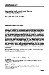
The starting values are P 00 (t ) = 1 and P 11 (t ) = 3u . From them one can proceed through the diagonal terms (m = n) by means of (2.5) to a P nn (t ) . The next terms, P n +1, n or P m,m −1 necessary to initialize the previous recurrence relations (2.6) and (2.7), can be obtained by the same relations (2.6) and (2.7) taking into account the fact that the constants the ALFs don’t exist to m>n and bn +1, n = h m ,m −1 = 0 in these cases. Then one can go ‘forward’ increasing sequentially the degree n in (2.6), or decreasing sequentially the order m in (2.7) (cf. Fig. 2.1). That is the reason why, following Holmes and Featherstone (2002), we have named these recursive relations ‘Forward Column’ (FC) and ‘Forward Row’ (FR) recursive methods respectively.
Degree n
Degree n
Order m Order m Fig. 1.1 Row and column schematic recursion procedures
There are equivalent recurrence relations for the derivatives of ALFs. For our purpose we only need the first derivatives. The corresponding FC and FR
hnm =
( n2 − m2 )(2 n + 1) , (2n − 1)
(2.11)
(n + m + 2)(n − m − 1) . ( n − m )(n + m + 1)
(2.12)
The calculus of the equal index terms, P 'nn (t ) , for the first derivatives ALFs is obtained from the following equation: t P 'mm (t ) = m P mm (t) . u
(2.13)
This equation can be deduced from the first derivative of (2.5) or from (2.9) considering that f mm = 0 . One of the biggest difficulties in dealing with the ALFs is that their absolute values range over thousands of orders of magnitude. For a degree M = 2700, P nm (t ) range over ∼5000 orders of magnitude when θ → 0o or θ → 180o (cf. Holmes and Featherstone, 2002). The IEEE standard 754 for a binary floating-point arithmetic only allows a representation of numbers ranging, in absolute value, between 10 −310 and 10 +310 approximately (cf. e.g. Overton, 2001), that is to say with a maximum range of ∼620 orders of magnitude. Outside these values numerical underflow or overflow occurs. When an underflow happens the computed value is set to zero giving erroneous results, and in the overflow situation any computed values are designated as NaN, giving no results at all. As a consequence of the u m = sin m θ term in (2.5) the diagonal terms decrease rapidly when m increases, particularly near the poles and there can be underflow. This is an especially grave situation, because when this happen these diagonal ones and all the other terms calculated from it are also set to zero, even when the terms outside diagonals, that grow forwards, should generate height values.
(
)
Normalization has been the common way to reduce the orders of the magnitude that ALFs range, and hence to mitigate this problem of underflow and overflow. The classical kinds of normalized ALFs used up to now have been adequate to treat the EGMs currently in use. These EGMs are complete up to a degree of 360 and with the IEEE 754 norm and adequate recurrence relations, neither overflow nor underflow takes place between latitudes ± 83 o , even with very small consequences when underflow happens inside these higher latitudes. Another complementary way to deal with this problem is to scale the ALFs when an underflow is about to occur (cf. Koop and Stelpstra). With this normalization and scaling techniques Wenzel (1998) could determine ALFs up to a degree and order M = 1900 for : 20o ≤ θ ≤ : 160o , using it to generate a tailored geoid for Europe. The proposed method by Libbrecht (1985), reviewed and generalized by Holmes et al. (2002), to prevent underflow when handling very high degree ALFs is to modify the recurrence relations (2.6), (2.7), (2.9) and (2.10), introducing in them a modified ALF defined as: ( P nm (t ) Pn m (t ) = . um
(g
nm
)
tPˆn ,m +1 (t ) − hnmu 2 Pˆn , m + 2 (t ) , (2.17)
(
1 Pˆ 'nm (t ) = ntPˆnm (t ) − f nmqPˆn −1,m (t ) u t Pˆ 'nm (t ) = m Pˆnm − enm uPˆn , m + 1 u
)
(2.18)
(2.19)
These are the equations -the Modified Forward Column (MFC) and Modified Forward Raw (MFR)- we are going to experiment with in order to determine the most appropriate one to use in the program. Once we have calculated the modified ALFs Pˆnm (t ) , or its derivatives, through one of the equations (2.16), (2.17), (2.18) or (2.19), we can use Horner’s schema of summation to make the summation of (2.2), or the equivalent one corresponding to the gravity quantity to be calculated (cf. Holmes and Featherstone, 2002): M
M
n= µ
n= µ
ˆ = cos mλ C nm Pˆ (t ) + sin mλ S n m Pˆ (t ). (2.20) Ω m ∑ ∑
(2.14)
(2.16)
)
}
}
It is easy to arrange this way of operating in order to obtain the other related gravity quantities, all of them connected to V through the following formulas:
T γ 1 ∂T ξ =− γ r ∂ϕ
W = V + φ ; T =V − U ; ∂T 2 − T; ∂r r 1 ∂T η=− , γ r cosϕ ∂λ
∆g = − (2.15)
{ ({
GM ˆ u+Ω ˆ M −1 u + Ω ˆ M −2 u+ ........ Ω M r ˆ2 u+Ω ˆ 1 u + GM Ω ˆ 0. ..... + Ω (2.21) r
V (r ,θ ,λ ) =
Then, we can obtain simultaneously the modified ( ALF Pnm (t ) multiplied by the q n factor in the recursive formulas. Effectively substituting (2.15) into (2.6), (2.7), (2.9) and (2.10) one obtains new recurrence relations: Pˆnm (t ) = anm qtPˆn −1,m ( t ) − bnmq 2 Pˆn − 2, m (t) ,
j
The Horner’s schema to sum (2.2) is given by:
By doing that the small values connected with the u m in (2.4) are avoided. But now, as a consequence, ( this Pn m (t ) can overflow. To prevent these situations it is necessary to have a posterior scaling of all the computation downwards by a global scale factor. Using a global scale factor of 10 −280 one can ( compute all Pn m (t ) up to a degree and order of 2700 without neither overflow or underflow. To reduce the computing time we can introduce a modified ALF defined as: n ( a ( Pˆnm (t ) = Pnm (t ) = q n Pnm (t ) r
1 Pˆnm (t ) =
ζ=
(2.22)
where φ is the potential of the centrifugal force, U is the normal gravity potential and γ the normal gravity (cf. equations (2.3), (2.61) and (2.114) of Heiskanen and Moritz, 1967). As we have already said the other algorithm we have tested to decide which one of them to implement is Clenshaw’s summation method. This
algorithm can evaluate the sums to appear in the calculus of the gravimetric quantities without evaluating the ALFs. It hasn’t therefore any instabilities. The basic idea of this method (cf. Gleason, 1985; Deakin, 1998) will be described below. We can arrange the (2.2) such that: V (r ,θ ,λ ) =
GM r
M
∑ ( cos mλ ) v + ( sin mλ ) v m c
m s
m=0
(2.23)
with: n
m m T a vcm = ∑ C nm Pn m (t ) = ∑ C n m P%n m (t ) = C P% n= µ r n =µ (2.24) n m m T a m % % v s = ∑ S nm Pn m (t ) = ∑ S nm Pnm ( t) = S P n= µ r n =µ
T −1 vcm % T ( A ) C % T c = P0 = P0 −1 vsm s ( AT ) S
(2.27)
where: c mm smm m m −1 c −1 s c = ( AT ) C = m•+1 and s = ( AT ) C = m•+1 (2.28) • • m m c M sM
and introducing (2.28) into (2.27) yields: % ( t) vcm = ∑ C nm P%nm (t ) = cmm P mm m
n= µ m
%mm ( t) v = ∑ S n m P%nm (t ) = sm m P m s
(2.29)
n= µ
n
a with P% (t ) = P ( t) . We can arrange also the r recurrence relations (2.16) and (2.5) in the following ways: nm
nm
P%nm (t ) − a% nm (t ) P%n −1,m (t ) + b%nm P%n −2, m (t ) = 0
(2.25)
where a% nm (t ) = qanmt is a linear function of t and b%nm = q 2 bn m is independent of t. For m ranging into
0 ≤ m ≤ M the recurrence relations formula (2.25) can be represented in matrix form as: 1 0 0 −a% ( t ) 1 0 m + 1 , m b% −a%m+ 2, m (t) 1 m+ 2,m 0 b%m+ 3,m −a%m +3, m (t) 0 0 .
0 0
0
0
1 .
0 .
0 0 0 0 0 0 0 0 . . . 1 0 0 −a%M −1, m (t) 1 0 b%M , m −a%M , m (t) 1
b%M −1, m
or
%
%
0
AP=P
P%m, m (t ) P%mm (t ) % Pm+ 1, m (t) 0 . . = . . P% 0 (t ) M − 1, m P%M ,m (t ) 0
0 0
0
0
0
0
(2.26)
Now, from (2.26) we have P% = A -1 P% 0 , and taking into account that vcm (and vsm ) are scalar quantities, and as a consequence they are equal to its transpose, (2.24) can be written as:
Then the summation of the products of the coefficients C nm or S nm and the modified ALFs is the product of a singular number cmm or smm and only the modified ALFs of degree and order m. But observing the pattern of the matrix A, together with the assignment of cM + 2 ,m = cM +1,m = sM +2 ,m = sM +1,m = 0 , we find that the elements of the vectors c and s are related by means of the following recurrence equations: cnm cn +1, m % c n +2, m C nm = a%n +1, m (t ) s − bn + 2, m s + . (2.30) snm n +1,m n +2, m S nm
From (2.30) we can obtain recursively the constants cmm or smm needed in (2.29). This is the recursive Clenshaw’s summation method. But the second sum (in the order m) in (2.2) can be also evaluated by a second implementation of Clenshaw’s recursive summation method. Effectively, introducing (2.29) into (2.2) yields: V (r ,θ ,λ ) =
GM r
M
∑ ( cos mλ ) c
m =0
mm
% . (2.31) + (sin mλ ) smm P mm
If we define: Ymm = ( cos m λ ) cmm + ( sin mλ ) s mm ,
(2.32)
and we introduce (2.32) into (2.31), and reverse the order of the summations, we obtain:
V (r ,θ ,λ ) =
GM r
0
∑Y
m =M
P% .
mm mm
(2.33)
This equation (2.33) is equivalent to any of the (2.24), and for its sum we can use the same reasoning used before. In this case we begin with the modified recurrence relation (2.5): P%m ,m ( t ) + a%mm (t )P%m −1,m −1 = 0
for integer values of θ ranging between 0o ≤ θ ≤ 180 o and 1o ≤ θ ≤ 179 o respectively. We have developed three different methods to calculate the sums (3.1) and (3.2): the MFC, the MFR and Clenshaw’s methods (CLE). The first test made was to calculate the relative numerical precision (cf. Holmes and Featherstone, 2002):
(2.34)
RP =
and this yields a similar equation as in (2.29):
to zero and the SHCs replaced by the Ymm values obtained by the first application of Clenshaw’s summation:
ym ,m = a% m +1, m ym +1, m + Ymm
(2.36)
As we can see it is possible to evaluate the formula (2.2) without calculating any ALF. The results here obtained can be easily extended to calculate the derivatives of the ALFs. For a detailed deduction of these formulas see the already cited papers of Gleason (1985) or Deakin (1998).
3. Testing the Different Algorithms We have made tests to check which of these algorithms is the most adequate to be implemented to calculate gravity quantities from a high degree SHC (to a degree and order of 2700) in a program running under Matlab™. To make comparisons with results obtained by other researchers we have used the methodology established by Gleason (1985), and from then on by many others such as Holmes and Fearesthone (2002), whose results we want to compare with our own. The way to operate is based on the calculus of sums of the ALFs:
Log. of rel. precision
where y00 can be obtained from a similar relation to that given in (2.30), but now the constants b% are set
(3.3)
where S(double) is the value of sums (3.1) or (3.2) in double precision for each method and S(extended) are the same sums with extended double precision (p = 64) format, permitted in Matlab™ (cf. Overton, 2001). We have made the assumption that in extended double precision we have obtain at least one significant figure more than those obtained in IEEE double precision. CLE were used as control values following Holmes and Featherstone (2002), who justified it stating this is ‘the most widely used method in geodesy’… and ‘can be used as a benchmark against which performance of the other methods’. -10
A
-12 -14 -16 0
Log. of rel. precision
(2.35)
-10
Log. of rel. precision
P% = y00 P%00 = y00
mm mm
m= M
-10
Log. of rel. precision
0
∑Y
S (double) − S (extended) S (extended)
-10
20
40
60
80
100
120
140
160
180
100
120
140
160
180
100
120
140
160
180
120
140
160
B
-12 -14 -16 0
20
40
60
80
C
-12 -14 -16 0
20
40
60
80
D
-12 -14 -16 0
Fig
20
3.1
40
60
Logarithm
80 100 Spherical Polar Distnce (Degree)
of
the
relative
precision
180
of
2700 n ∑n =0 ∑ m= 0 P nm (cos θ ) using MFC (A) and MFR (B) together with Clenshaw’ method (dashed lines), and logarithm of the relative precision of 2700 n ∑n =0 ∑ m= 0 P ' nm (cosθ ) , using MFC (C) and MFC (D) and Clenshaw’s method (dashed lines).
2700 n
S = ∑ ∑ P (cos θ ) n= 0 m = 0
(3.1)
nm
or their derivatives:
S'=
2700 n
∑∑P'
nm
n =0 m =0
(cos θ ),
(3.2)
As seen in Fig 3.1 the MFR methods, which correspond with the graph (B) and (D), have more relative precision in the calculus of the sums of ALFs and their first derivatives, especially near the poles. To determine the accuracy of our methods the two following well-known identities were used:
∑ ∑(P
(cos θ ) nm
∑ ∑ (P '
)
M
n
n =0 m = 0
M
)
2
= ( M + 1) 2 ,
nm
(cos θ )
n= 0 m = 0
M ( M + 1) ( M + 2 )
(3.4)
2
2
n
∀θ
=
4
(3.5)
,
both valid for (0o < θ < 1 8 0o ) . When M = 2700 the values in the right hand side of (3.4) and (3.5) are 7 295 401 and 13 305 717 113 850 respectively. Then we calculate the relative numerical accuracy of each algorithm as:
NAP =
(
(
)
)
2700 M 2 ∑ ∑ P nm (cos θ − 7 295 401 n =0 m =0
(3.6)
7 295 401
M 2 2700 ∑ ∑ ( P 'nm (cos θ ) − 13 305 717 113 850 n =0 m =0 NAP ' =
(3.7)
13 305 717 113 850
Logarithm of relative accuracy
-12.5
-13
Ta ble 1. Efficiency of the MFC, MFR and CLE algorithm 1.67 MHz 490 Mhz Ec. (3.1) Ec. (3.2) Ec. (3.1) Ec. (3.2) (s) (s) (s) (s) MFC
41.52
69.67
211.70
384.49
MFR
115.34
136.45
273.64
520.58
106.33
170.55
247.36
498.90
CLE
-13.5
-14
A -14.5
-15 60
70
80
90
100
110
120
70
80
90 Spherical polar distance (degree)
100
110
120
-12 Logarithm of relative accuracy
these near polar values. This is not new because Wiggins and Saito (1971) have already stated that the forward row recurrence relation (2.7) ‘show almost no loss of significance for all values of n, m and θ ’. Nevertheless this relation has hardly been used in geodesy due the general belief that the presence of u (=sinθ ) in the denominator of (2.7) should make it impractical (cf. Koop and Stelpstra, 1989). The next test concerns efficiency. The first one consisted in calculating the necessary times to sum up to a degree of 2700 the Ec.3.1, corresponding to ALFs and the sum of their first derivatives (Ec. 3.2) in a PC with a microprocessor running at 1.67 GHz and on a laptop running at 490 MHz.
-12.5 -13
As we can see in Table 1, the most efficient algorithm is the MFC, and the slowest one is the MFR.
-13.5 -14
B -14.5 -15 60
Fig. 3.2
Logarithm of relative accuracy of :
∑n (A) ∑ 2700 n = 0 m = 0 ( P nm (cos θ ) ) using MFC (solid line) and 2
∑n MFR (dashed line)and (B) ∑ 2700 n = 0 m = 0 ( P ' nm (cos θ )) using . MFC (solid line) and MFC (dashed line). 2
In the calculus of accuracy through (3.6) and (3.7), the range of values were restricted to 60o ≤ θ ≤ 120o because it is not possible, outside them, to obtain the sum of the square of the ALFs nor the squares of their derivatives in IEEE double precision without underflow. As we can see in Fig.3.2, the MFC algorithm produces a bit more accuracy in the range of values used for our calculus, for both ALFs and for their first derivatives. Holmes and Featherstone (2002) have extended their calculus in all the range of latitudes and have proved that near the poles the situation is inverted and that the MFR is more accurate for
Table 2. Time of calculus of different programs. 1.65 GHz 490 MHz 200 MHz
MFC
MFR
CLE
R
G
A
14.9
17.3
13.4
-
-
-
37.7
72.4
53.6
-
-
-
-
-
-
4942
368
101.5
Table 2 compares our results with those published by Abd-Elmootaal (1997). To do this, the same gravity quantity was calculated ∆g , using the same model EGM96, and also on a grid of 0.5o × 0.5 o for all the Earth. This table estimates the time of the calculus with the algorithms MFC, MFR, CLE, and with the programs of Rapp (R), Geocol (Tscherning), (G) and Abd-Elmootal (A), with data published by Abd-Elmootal (1997). To determine the time these algorithms will take to calculate the gravimetric quantities with a very
high geopotential model we have used Kaula’s rule to calculate synthetic SHC from a degree and order 360 to 2700 and to extend the EGM96 to degree of 2700. The results of the calculation of some gravimetric quantities with different algorithms on a PC running at 1.65 GHz are given in Table 3. These gravimetric quantities have been calculated simultaneously on a grid of 1o × 1o for all the Earth. Table 3. Time in seconds of some gravimetic quantities with a simulate geopotential model of a degree and order of 2700 in a grid of 1o × 1o for all the Earth. N
∆g
ξ
η
MFC
118.0
119.5
138.6
118.4
MFR
146.5
153.7
189.5
149.3
CLE
136.4
145.3
168.9
139.2
4. Conclusions As a consequence of the results obtained in the previous sections, we have selected for the definitive version of our program the MFC algorithm. This is faster than the other ones when it is implemented in Matlab™. We have used efficiency as the criterium due to the difference amongst all of them in accuracy not being significant. Being Matlab™ an interpreted language, the necessary constants can be easily modified in our program in order to express the results in a determinate permanent tide system, reference ellipsoid, or a specified value of the potential (cf. Smith, 1998).
References Abd-Elmotaal H.A. (1997). An efficient technique for the computation of the gravimetric quantities from geopotential earth models. Proc. of IAG Scientific Assembly, 3-9 September, Rio de Janeiro. Clenshaw, C.W. (1955). A note on the summation of the Chebyshev series. Math Tab Automat Comput 9: 118-120. Colombo, C. (1981). Num erical methods for harmonic analysis on the sphere. Rep 310, Department of Geodetic Science and Surveying, OSU, Columbus. Deakin, R.E. (1998). Derivatives of the Earth’s potentials. Geom Res Aust 68: 31-60. Gleason, D.M. (1985). Partial sums of Legendre series via Clenshaw summation. Manuscr Geod 10: 115-130. Heiskanen, W.A. and H. Morittz. (1967). Physical geodesy, Freeman, San Francisco. Higham, D.J. and N.J. Hogham. (2000). Matlab guide. Siam .Philadelpia. Holmes, S.A. and W.E. Featherstone. (2002). A un ified pproach to the Clenshaw summation and the recursive
computation of very high degree and order normalised associated Legendre functions. Journal of Geodesy 76 pp.:279-299. Koop, R. and D Sptelpstra (1989). On the computation of the gravitational and its first and second order derivatives. Manuscripta Geodaetica. Nº 14 pp.:373-382. Libbrecht, K.G. (1985). Practical considerations for the generation of large order spherical harmonics. Solar Phys 99: 371-373. Lundberg J.B. and B.E. Schutz. (1988) Recursio n formulas of Legendre functions for use wit h non-singular geopotential models. J. Guidance. Vol. 11, n 1 pp. 31-38. Magnus, W., F. Oerhettinger and R.P. Soni. (1966). Formulas and theorems for special functions of mathematical physics, 3rd edn. Springer, Berlin, Heidelberg, New York. Overton, M.L. (2001). Numerical computing with IEEE Floating Poin Arithmetic. Siam, Philadelphia. Pavlis, N.K., S.A. Holmes. S. Kenyon, D. Schmit, R. Trimmer. (2004) Gravitational potential expansion to degree 2160. IAG International Symposium, gravity, geoid and Space Mission GGSM2004. Porto, Portugal. Rapp, R.H. (1997). Use of potential coefficient models for geoid undulation determinations using a spherical harmonic representation of the height anomaly/geoid undulation difference. J of Geodesy 71:282-289. Rizos, C. (1979). An efficient computer technique for the evaluation of geopotential from spherical harmonic models. Aust J Geod Photogram Surv 31: 161-169. Tscherning, C.C. and K. Poder. (1982). Some geodetic applications of Clenshaw summation. Boll Geofis Sci Aff 4: 351-364. Tscherning, C.C., R.H. Rapp., and C. Goad. (1983). A comparison of methods for computing gravimetric quantities from high degree spherical harmonic expansions. Manuscr Geod 8: 249-272. Sanso, F., and G. Sona (2001 ). ELGRAM: an Ellipsoidal Gravity Model Manipulator. Bull. Geod. Sci. Affini. 60, 3, pp.:215-226. Smith, D.A. (1998). There is not such thing as “The” EGM96 geoid: Subtle points on the use of a global geopotetial model. IGeS Bulletin Nº 8, pp. 17-28, Milan, Italy. Wenzel G. (1999). Ultra High Degree Geopotential Models GPM98A and GPM98B. Bolletino di Geofisica Teorica ed Applicata . Wiggins, R.A. and M. Saito, (1971) Evaluation of computational algorithms for the associated Legendre polynomials by interval analysis. Bulletin of the Seismological Society of America. Vol 61 nº 2, pp. 375381.


![[PDF] Optimization Using Personal Computers - Google Sites](https://m.moam.info/img/260x300/pdf-optimization-using-personal-computers-google-s_6478e9a1097c4796708d54b5.jpg)