Using supervised training signals of observable state dynamics to speed-up and improve reinforcement learning Daniel L Elliott
Charles Anderson
Dept of Computer Science Colorado State University Email:
[email protected]
Dept of Computer Science Colorado State University
Abstract—A common complaint about reinforcement learning (RL) is that it is too slow to learn a value function which gives good performance. This issue is exacerbated in continuous state spaces. This paper presents a straight-forward approach to speeding-up and even improving RL solutions by reusing features learned during a pre-training phase prior to Q-learning. During pre-training, the agent is taught to predict state change given a state/action pair. The effect of pre-training is examined using the model-free Q-learning approach but could readily be applied to a number of RL approaches including model-based RL. The analysis of the results provides ample evidence that the features learned during pre-training is the reason behind the improved RL performance.
I.
I NTRODUCTION
The promise of reinforcement learning (RL) is that an agent can be taught to learn some behavior by supplying it with a (potentially incomplete) representation of its current state and only a scalar-valued feedback representing the quality of its performance as a training signal. This stands in contrast to the supervised learning approach where the agent is taught from a set of sample training states providing the preferred action for every state as the training signal. In the RL approach the agent learns by exploring its environment and the, sometimes, many approaches to solving a given problem. It frees the human trainers from having to know the preferred action or intrinsic value of each encountered state. There is no denying that RL has a grassroots feel: is an important form of learning in the natural world and it is only natural that machine learning practitioners would want to mimic its success. This freedom comes at a price, however. One common complaint is that RL is too slow to converge. In a continuous domain, the types of which are all around us, slow convergence can be exacerbated by the size of the state space. This paper presents results pointing to a simple, yet powerful, approach for improving the speed by which the RL agent will find quality solutions. In the opening paragraph of their foundational book on RL, Sutton and Barto, [1], posit that interaction with one’s environment is at the very core of learning. Interestingly, the example they use, an infant’s first few months’ experiences within the world, describes no purpose to the actions performed by the baby, only that the baby has access to a wealth of information about cause and effect. Learning cause and effect is not the
primary purpose of RL, even if it is a requisite aspect. In practice, supervised learning is more apt to learn those types of relationships. Likewise, as an agent interacts with its environment, similar information about its world is available. The approach presented in this paper, dubbed pre-training, is to take advantage of ancillary information – ancillary to the RL reward signal – from the environment and to use it to pre-train the RL agent to learn a quality solution with less computation. As discussed in Section II, utilizing information gathered through interaction with the environment is not a new concept. For years, models created from this data have been used along side value functions in model-based RL approaches. In this work, pre-training is tested using a few variations of a simulated marble track where the goal is to move a marble into the goal region as quickly as possible and to keep it there as long as possible. This problem domain has a continuous state space with discrete actions. The agent solves this problem using the Q-learning approach to RL via an artificial neural network (ANN) [2]. The novel aspect of this approach is that, prior to using Q-learning to adjust the ANN weights, the hidden layer of the ANN is pre-trained by initializing the hidden unit weights by including them as a part of another ANN trained to predict the dynamics of the marble track via supervised learning. Pre-training is simply training the ANN to predict the change in position and velocity given the current state and action prior to beginning RL. No additional information is provided during pre-training beyond what would be available in the state description used as inputs during RL. Specifically, no goal-related information is included during pre-training. When might features learned in a model be useful in learning a value function? An obvious case is real-world problems for which the minimum set of state variables is not known, so many sensed measurements are included in the hope that they collectively provide sufficient context for the RL agent to learn successful policies. A model trained in this case will learn representations composed of just the critical variables— ones unrelated to the dynamics of the environment. Without the proposed pre-training, an RL agent must search for good policies and good representations. With pre-training the effort of searching for good representations may be much reduced. Other cases where pre-training is expected to help is when
both the model and the RL agent require nonlinear features, such as trigonometric functions, of the original variables. The results show that pre-training the hidden layer weights reduces the number of trials necessary for the agent to find a quality solution when compared to Q-learning without pretraining. Furthermore, in some experiments, the solutions found via pre-training are superior to the solutions found without pre-training. Finally, our analysis indicates that, as expected, the improved performance with pre-training is a result of those hidden units modeling important features of the marble track problem. The remainder of this paper includes the following sections. Section II summarizes published work that is related to the approach described here. Section III provides a background to reinforcement learning and function approximation with neural networks and introduces the pre-training approach. Section IV describes experiments with a simple reinforcement learning problem consisting of a simulated point mass with velocity moving in several one-dimensional environments with increasing difficulty. Section V discusses an analysis of hidden unit activations as a new way to investigate the hypothesis that representations developed during pre-training facilitate the learning of value functions during reinforcement learning. Section VI summarizes conclusions and future work. II.
R ELATED WORK
The Dyna-Q [1] RL approach utilizes data collected during interactions with the environment to build a model of the environment. The model is used to simulate additional interactions which are used to create additional, high-speed trials to speedup Q-learning. More recently, Deisenroth, et al.,[3], used data collected during RL to learn a model of environment dynamics in a model-based approach. In their work, separate Gaussian process models are fit to the value function and the model of the environment. Like in the approach presented here, the data set used to learn the environment model is generated prior to learning the value function. Unlike the approach presented here, there is no reuse of features learned during environment dynamics training. The predictive state representations (PSR) approach has received attention as a method of using data collected during interactions with the environment to improve RL and has been extended to continuous states and actions [4]. PSRs represent state using probabilities of experiencing a sequence of observation/actions pairs given a history of such pairs. It appears that the continuous extension to PSR would require a greatdeal of complex processing. Despite PSR’s well developed theoretical foundation, they have not found wide-spread usage in the literature. State prediction is utilized in the multiple module RL approach (MMRL) [5]. In MMRL, state prediction is not used to improve the value function, as it is with pre-training, but is used to partition the state space using a mixture of experts approach. A separate value function is learned for each partition. Kormushev and Caldwell, [6], included some state information along with the reward in a continuous state/action archery
simulation. However, the state information used to augment the reward (called multi-dimensional feedback) was the 𝑥, 𝑦 offset of the arrow from its intended target. They then use a specialized RL algorithm to prefer parameter updates which will improve the simulated 𝑥, 𝑦 offset. This method supplies their approach with additional, goal-related information which is distinctly avoided in the approach presented in this work. Ni, et al., [7], achieved faster RL using ANNs via an actorcritic approach on a discrete maze navigation simulation. They did this by adding a third ANN, two already present for the actor and critic, called the goal network, which is trained to learn the total, discounted reward given a state/action pair. The critic is trained to emulate the output of the goal network. According to the authors, the advantage of the goal network is that it provides immediate feedback at every time step instead only in specific states. None of the existing methods reviewed above for incorporating experiential data via interaction with the environment do so by pre-training. Our pre-training approach can be combined with any of the reviewed methods, such as the use of the pre-trained model to generate additional interaction data by simulation. In this paper the use of ancillary data gathered while interacting with the environment in a model-free RL algorithm is investigated. Dynamics data is used extensively in model-based RL which uses a model of the environment to predict future states. In certain domains the model used in model-based RL can be learned from data collected during interactions with the environment. The approach explored here is model-free. The quality of the environment dynamics prediction during pretraining is not at issue. Model dynamics are only learned as a device for initializing the Q-learning ANN hidden units to improve Q-learning. III.
R EINFORCEMENT L EARNING WITH N EURAL N ETWORKS AND P RE -T RAINING
Sutton and Barto, [1], describe a reinforcement learning approach as requiring three elements: a policy that defines the agent’s behavior by mapping the perceived state of the agent within the environment to an action, the reward function which defines the goal, and a value function which computes the amount of reward an agent can expect to accumulate by taking a specific action at a specific state. In short, the reward function specifies the immediate value of a state while the value function computes the long-term value of a state. Many times, as in the approach presented here, the policy utilizes the value function in selecting an action given a state. Some RL approaches utilize a model of the environment. However, a model-free approach is explored in this work. The majority of the effort required to utilize a RL approach is typically encountered in learning the value function [1] and this is the case in the approach presented here. The experiments presented here utilize Q-learning to learn the value function. Because the state space is continuous, an ANN is used to model the value function. Q-learning is an off-policy, temporal-difference approach to RL [1]. In Q-learning, the value function is approximated using the Q-function which maps state/action pairs to an estimate
of the value. The Q-function is updated through repeated interaction with the environment according to (1). [ 𝑄(𝑠(𝑡), 𝑎(𝑡)) ← 𝑄(𝑠(𝑡), 𝑎(𝑡)) + 𝛼 ] 𝑟(𝑡 + 1) + 𝛾 max (𝑄(𝑠(𝑡 + 1), 𝑎′ )) − 𝑄(𝑠(𝑡), 𝑎(𝑡)) (1) ′ 𝑎
where 𝑡 is the current time step, 𝑄(𝑠(𝑡), 𝑎(𝑡)) is the Q-function value for state/action pair (𝑠(𝑡), 𝑎(𝑡)), 𝑠(𝑡+1) is the state which occurs when taking action 𝑎(𝑡) from state 𝑠(𝑡), 𝑟(𝑡 + 1) is the reward at time 𝑡 + 1, 𝛼 is a learning rate parameter, and 𝛾 is a parameter modulating the effect of future rewards. The value max𝑎′ (𝑄(𝑠(𝑡 + 1), 𝑎′ )) is the current estimate of future reward: it represents the best possible action, 𝑎′ , taken at the next state, 𝑠(𝑡 + 1). Using an ANN with backpropagation to model a Qfunction is a common method when applying Q-learning to continuous domains [2]. Here, the ANN models the Q-function by taking state and action as inputs and outputting a single (𝐷) value. The notation of the ANN is that 𝑊𝐻 and 𝑊𝐻𝑂 are the hidden and output layer weight matrices of the dynamics (pre(𝑄) training) ANN and 𝑊𝐻 and 𝑊𝐻𝑂 are the weight matrices of the ANN trained using Q-learning. Both ANNs share the 𝑊𝐻 weights with separate output layers. Pre-training is performed by including 𝑊𝐻 as a hidden layer in an ANN which is trained to predict state dynamics (i.e. position and velocity change) via supervised learning. The hidden layer activations are denoted as 𝑧 and the dynamics and Q-function ANN output activations are denoted as 𝑦 and 𝑞 respectively. The ANN activation functions are 𝑡𝑎𝑛ℎ with the exception of the output layer of the Q-function ANN which is linear. IV.
E XPERIMENTS
Three different marble track domains (a flat track, a hilly track, and a track with a region of negated action, are used to explore the potential benefit of preforming pre-training. In the following sub-sections, they are presented in order of perceived difficulty. A. Marble track domain The concept of pre-training was explored using a simulated, 1-D marble track. The goal of this exercise is for the learner to keep the marble in the goal area while staying within a velocity range. The learner can manipulate the marble’s velocity by pushing the marble right or left or taking no action. In all experiments, the state at time 𝑡 consists of position and velocity: 𝑠(𝑡) = (𝑠𝑝 (𝑡), 𝑠𝑣 (𝑡)) , 𝑠𝑝 ∈ [0, 10], 𝑠𝑣 ∈ [−5, 5]. The simulation incorporates friction and gravity. If 𝑠𝑝 exceeds the valid range, 𝑠𝑝 is set to the nearest extreme value (zero or ten) and 𝑠𝑣 is set to zero to simulate collision with a barrier. The reward, 𝑟, is zero if the state is within the goal and negative one otherwise. All ANN inputs are scaled into [−1, 1]. Initial ANN weights are randomly, uniformly drawn from [−0.4, 0.4]. Algorithm 1 describes the algorithm for computing 𝑠(𝑡+1) given 𝑠(𝑡) and 𝑎(𝑡). Algorithm 1 has several configurable parameters. The slope of the track at position 𝑝 is represented by 𝜃𝑝 , P𝑑 is the set of negated-action regions defined by start and end positions pairs: (𝑝𝑠 , 𝑝𝑒 ), Δ𝑇 = 0.1 is the Euler integration time step, 𝑓𝑐 = 0.1 is the friction coefficient, and 𝑀 = 1 is the ball mass.
Algorithm 1: Marble track dynamics algorithm. if 𝑠𝑝 (𝑡) ∈ [𝑝𝑠 , 𝑝𝑒 ∀𝑝∈P𝑑 ] then 𝑎(𝑡) ← −𝑎(𝑡); 2 𝑔(𝑡) ← 𝑀 × sin(𝜃𝑝 ); 3 𝑓 (𝑡) ← 𝑓𝑐 × 𝑀 × 𝑠𝑣 (𝑡); 4 𝑠𝑣 (𝑡 + 1) ← 𝑠𝑣 (𝑡) + Δ𝑇 × (𝑎(𝑡) + 𝑔(𝑡) − 𝑓 (𝑡)); 5 Bound 𝑠𝑣 (𝑡 + 1) within [−5, 5]; 6 𝑠𝑝 (𝑡 + 1) ← 𝑠𝑝 (𝑡) + Δ𝑇 × 𝑠𝑣 (𝑡 + 1); 7 if 𝑠𝑝 (𝑡 + 1) ∈ / [0, 10] then 8 𝑠𝑣 (𝑡 + 1) ← 0; 9 Bound 𝑠𝑝 (𝑡 + 1) within [0, 10]; 10 end 1
In Algorithm 1, step 1 is the negated-action region calculation. Step 2 is the gravity calculation which is influenced by the slope, 𝜃𝑝 . Step 3 computes the friction between the marble and the track. Step 4 computes the new velocity which immediately determines the next position in step 6. Steps 7–10 handle the track boundary scenarios. Algorithm 2 presents the pseudo code for the algorithm used in these experiments to perform Q-learning and pretraining using an ANN. In these experiments, the configurable parameters associated with the learning algorithm implementation are the number of Q-learning trials (𝑁𝐽 ), the length of each trial (𝑁𝑇 ), and the number of pre-training epochs (𝑁𝐷 ) over the dynamics training data set (X , Y ). The pre-training input data, X ∈ 𝑀3,4920 , is drawn from a grid of 4920 points spaced throughout the three-dimension state space of valid (𝑠𝑝 (𝑡), 𝑠𝑣 (𝑡), 𝑎(𝑡)) tuples. The pre-training target data, Y ∈ 𝑀2,4920 , is the resulting change in state: (𝑠𝑝 (𝑡 + 1) − 𝑠𝑝 (𝑡), 𝑠𝑣 (𝑡 + 1) − 𝑠𝑣 (𝑡)). During RL, the learner spends most of its time at lower velocities (2.5 or less) so the 𝑠𝑣 values of X are spaced logarithmically in both the positive and negative directions starting at 𝑠𝑣 = 0. X is spaced evenly across 𝑠𝑝 values. A Q-learning trial is a single teaching episode starting at a randomly selected position and velocity and continuing for 𝑁𝑇 time steps. Q-learning adds the 𝛾 parameter [1] which is fixed at 0.95. During learning the 𝜖-greedy [1, p. 28] policy is used. The 𝜖-greedy policy selects the best action, as determined by the value function, with probability 1 − 𝜖. Otherwise the action is randomly selected. As Q-learning progresses, emphasis is shifted from exploration of the state space to exploitation of the learned value function by decreasing 𝜖. This strategy is called 𝜖-decay. In this implementation, the 𝜖 value is decayed at each time step of each trial according to: ( ) 𝜖𝑓 𝑖𝑛𝑎𝑙 𝜖(𝑡) ← 𝜖(𝑡 − 1) log . (2) 𝑁𝐽 𝑁𝑇 with 𝜖(𝑡 = 0) = 1.0 and 𝜖𝑓 𝑖𝑛𝑎𝑙 = 0.1. During value function evaluation, the policy is deterministic. This is equivalent to 𝜖 = 0. In Algorithm 2, steps 4–11 perform pre-training. Matrix notation is used here because these parameter updates are done in batch for the entire data set. Steps 13–26 represent a single trial and perform Q-learning. The Q-learning parameter updates are performed at each time step at step 26.
Algorithm 2: Pseudo-code for a single run (set of parameter values) of an experiment. 1 Set experimental parameters; 2 Generate dynamics data set inputs (X ) and target values (Y ) ; 3 Initialize ANN weights; 4 5 6 7 8 9 10 11 12 13 14 15 16 17 18 19 20 21 22 23 24 25 26 27 28
for 𝑑 ∈ {1, . . . , 𝑁𝐷 } do begin Forward pass through ANN 𝑍 ← tanh (X 𝑊𝐻 ); (𝐷) 𝑌 ← 𝑍𝑊𝑂 ; end Compute SSE between 𝑌 and Y ; (𝐷) Update 𝑊𝐻 and 𝑊𝑂 via backprop; end for 𝑗 ∈ {1, . . . , 𝑁𝐽 } do Initialize 𝑠(𝑡 = 1), 𝑎(𝑡 = 1); for 𝑡 ∈ {1, . . . , 𝑁𝑇 } do Compute 𝑠(𝑡 + 1) and determine 𝑎′ ; Compute 𝑟(𝑡); begin // 𝑄(𝑠(𝑡), 𝑎(𝑡)) computation. 𝑍 ← tanh ([𝑠(𝑡), 𝑎(𝑡)]𝑊𝐻 ); (𝑄) 𝑄(𝑠(𝑡), 𝑎(𝑡)) ← 𝑍𝑊𝑂 ; end begin // 𝑄(𝑠(𝑡 + 1), 𝑎′ ) computation. 𝑍 ← tanh ([𝑠(𝑡 + 1), 𝑎′ ]𝑊𝐻 ); (𝑄) 𝑄(𝑠(𝑡 + 1), 𝑎′ ) ← 𝑍𝑊𝑂 ; end // Compute error 𝛿(𝑡) ← 𝑟(𝑡+1)+𝛾𝑄(𝑠(𝑡+1), 𝑎′ )−𝑄(𝑠(𝑡), 𝑎(𝑡)); (𝑄) Update 𝑊𝐻 and 𝑊𝑂 via backprop; end end
Step 15 is the application of action 𝑎(𝑡) in state 𝑠(𝑡) to obtain state 𝑠(𝑡+1). Once 𝑠(𝑡+1) is determined, 𝑎′ is selected according to max𝑎′ (𝑄(𝑠(𝑡 + 1), 𝑎′ )) which is the best action from the next state according to the current Q-function. Step 16 is the reward calculation. Steps 17–20 is the computation of 𝑄(𝑠(𝑡), 𝑎(𝑡)) and steps 21–24 is the computation of 𝑄(𝑠(𝑡 + 1), 𝑎′ ) from (1). B. Flat marble track The initial experiment was carried out using a domain with little in the way of unobserved state. The flat marble track has no hills or regions of negated action. The hypothesis behind this experiment was that the learner will discover a good value function more quickly when pre-training is used. In this experiment, the goal is defined by a reward value of 0 as defined by the reward function { 0, if 𝑠𝑝 ∈ [4.25, 5.75] and ∣𝑠𝑣 ∣ < 0.8; 𝑟(𝑡) = −1, otherwise. Each run was 5 × 10⁴ trials in length. 𝑄 Each ANN layer has a configurable learning rate: 𝛼𝐻 = 𝑄 −3 −2 𝐷 −4 𝐷 1×10 , 𝛼𝑂 = 1×10 , 𝛼𝐻 = 1×10 , and 𝛼𝑂 = 1×10⁻⁵
𝑄 (e.g. 𝛼𝐻 is the learning rate for the hidden layer weights during Q-learning). The number of hidden layer units, 𝑀𝐻 , was fixed 𝑄 𝑄 , 𝛼𝑂 , 𝛾 and 𝑀𝐻 were set using a coarse at 15. Parameters 𝛼𝐻 parameter search to maximize the performance of Q-learning 𝐷 𝐷 without pre-training. Parameters 𝛼𝐻 and 𝛼𝑂 were set using a coarse parameter search to minimize the model error on the X data set.
Several values of 𝑁𝐷 were compared. Here 𝑁𝐷 ∈ {0, 2 × 10⁴ , 5 × 10⁴ , 1 × 10⁵ , 1.5 × 10⁵ , 2 × 10⁵ }. Each 𝑁𝐷 value was run 70 times. Each learning trial was 100 time steps in duration. Every 250 trials, the learned policy was evaluated by ¯ across 10 evenly-spaced starting computing a mean reward, 𝑅, positions with zero velocity and run for 200 time steps.
¯ value Fig. 1. Results from the flat marble track domain. Each line is the 𝑅 averaged over 70 runs for the given 𝑁𝐷 value. The “x” are plotted at intervals of 250 trials. The lightest line is no pre-training and the darkest line is the maximum amount of pre-training attempted.
¯ values averaged across 70 runs for Figure 1 shows the 𝑅 selected 𝑁𝐷 values. As expected the ANNs conditioned via pre-training learned better policies with a fewer number of trials than without pre-training. Figure 1 appears to show little benefit to an increased number of pre-training epochs after 𝑁𝐷 reaches 2 × 10⁴ . One interesting aspect of Figure 1 is the decrease in mean ¯ following the early, positive peak. This peak was a common 𝑅 feature across all experiments. This peak may be the result of the ANN diverging from a good Q-function after being trained for too long in the state spaces near the goal, causing the ANN to forget the Q-function outside the preferred state spaces. This is an aspect of utilizing an ANN to learn a Q-function and is not specific to the approach presented here. C. Hilly marble track It is expected that the presence of hills (unobserved state) will favor pre-training more than the flat marble track. Figure 2 shows the layout of the marble track. Figure 3 shows the results of this experiment. The results are similar to the flat track experiment with somewhat lower ¯ values. Also, the mean 𝑅 ¯ values eventually reach the mean 𝑅 highs seen in the peak region as learning continues. Finally,
Fig. 2. Hilly marble track. The goal region is the hatched region in the center of the track. The flat marble track has the same goal region with no sloped segments.
¯ curve for each 𝑁𝐷 value. The lighter line is the Fig. 4. Area under the 𝑅 same data as in Figure 1 and the darker line is the same as Figure 3. Each line from Figures 1 and 3 is condensed into a single point along one of these two lines. Notice the different y-axis scales for the two lines. The flat track values are computed from the first 12,500 trials and the hilly track values are computed from the first 25,000 trials. The number of trials to include is ¯ values for all trials up to and immediately after the selected to capture the 𝑅 peaked regions of each figure.
D. Marble world with region of negated action This experiment was carried out by negating the effect of actions when 𝑠𝑝 ∈ [6.5, 8]. The expectation was that this domain would be more difficult than the hilly domain and, therefore, would further highlight the advantage of pretraining. In this experiment the goal was 𝑠𝑝 ∈ [4.5, 5.25] and ∣𝑠𝑣 ∣ < 1.5. Also, 𝑀𝐻 = 10 and 𝑁𝐷 values of 0, 2 × 10⁴ , and 5 × 10⁴ were tested. Each run was 2 × 10⁴ trials in length. Otherwise, the experiment was run as described in Section IV-B. Figure 5 shows the positions of the goal and negatedaction region in this experiment. ¯ values plotted every 250 trials averaged over Fig. 3. Hilly track results. 𝑅 70 runs. Each line is a different 𝑁𝐷 value. The lightest line is no pre-training and the darkest line is the maximum amount of pre-training attempted.
there is a more gradual improvement when adding pre-training and this improvement appears to continue as 𝑁𝐷 increases. How does the size of the improvement from 𝑁𝐷 = 0 to 𝑁𝐷 > 0 compare between the flat and hilly marble tracks? Figure 4 relates the total reward experienced by the agent accross all trials to the amount of pre-training for the hilly and flat marble tracks. Figure 4 displays the area under the curve ¯ values shown in Figures 1 and 3) for the (the summed, mean 𝑅 flat and hilly tracks. The darker curve for the hilly track shows a more obvious, gradual increase in the area with increasing 𝑁𝐷 . The lighter curve shows the immediate advantage of pretraining and the diminishing returns of increasing the number of pre-training epochs. The percent increase of the area under the curve between 𝑁𝐷 = 0 and the 𝑁𝐷 with the highest area under the curve is 35.3% for the flat track and 49.2% for the hilly track.
Fig. 5. Negated action region experiment marble track. The goal region is the hatched region in the center of the track. The negated-action region is the region with the starred hatch pattern.
The results of this experiment are summarized in Figure 6. There is a clear trend of improved performance with increasing ¯ values 𝑁𝐷 : a good value function is found more quickly and 𝑅 are higher. In the 2 × 10⁴ trials, the 𝑁𝐷 = 0 version shows little promise of catching up with the 𝑁𝐷 > 0 versions. The 𝑁𝐷 = 5 × 10⁴ version begins making consistent improvement ¯ a full 5,000 trials before 𝑁𝐷 = 0 and the improvement in 𝑅 is much steeper. The results of this experiment are explored further in Section V. V.
H IDDEN NODE ACTIVATION ANALYSIS
Intuitively, the benefit of pre-training is that it conditions the hidden layer units to represent features beneficial to RL
¯ > −60 resulting in: is the set of trials with 𝑁𝐷 = 0 and 𝑅 𝑍 𝑔 = [𝑧1 (𝑡, 𝑗)∣𝑧2 (𝑡, 𝑗)∣ . . . ∣𝑧𝑀𝐻 (𝑡, 𝑗)∣ . . .] ∀𝑡∈𝑇,𝑗∈𝑁𝐽 ,𝑅>−60 ¯ (3) where 𝑍 𝑔 ∈ 𝑀1250,1530 and 𝑡 denotes the time step of trial 𝑗 for all runs with 𝑁𝐷 = 0. The number of PCs is limited to the dimension of 𝑍 𝑔 . In this case, there is a maximum of 1250 PCs.
Fig. 6. Results for the negated-action region experiment. The lightest line is no pre-training and the darkest line is the maximum amount of pre-training attempted.
Fig. 7. Example hidden node activations from the negated-action experiment. As in Figure 8, the y-axis is velocity and the x-axis is position. Images were created with 𝑎 = 0 as input which corresponds to the “do nothing” action. A lighter color represents a higher activation value.
before RL begins. In this Section principal component analysis (PCA) is used to examine this hypothesis. The authors are unaware of any previously published use of this method of analyzing ANN activations across state spaces. This method is useful to get a feel for the variations of activations across many ANNs instead of just looking at each hidden node’s activation individually. The PCA analysis shows
Many times some meaning behind a PC can be gleaned from inspecting the PC as an image. The PC dimensions correspond to the dimensions of the state activation image which enables viewing them as an image. Figure 8 shows the first ten PCs.
∙
the pre-trained hidden units begin Q-learning with activations which are closely related to good RL performance,
∙
the hidden units quickly increase in this association as the trials progress, and
∙
this association increases with increasing 𝑁𝐷 .
Data from the negated-region marble track experiment was used in this analysis. This analysis was performed by creating ¯ > −60. a PCA subspace from trials with 𝑁𝐷 = 0 and 𝑅 This selection represents the best-performing trials of runs without pre-training. A PCA subspace is created using the singular value decomposition (SVD). The SVD of a matrix, 𝑍, computes 𝑈 and 𝑉 where 𝑈 is a matrix whose columns are the eigenvectors of 𝑍𝑍 𝑇 [8]. 𝑍𝑍 𝑇 computes the covariance of the rows of 𝑍. The column vectors of 𝑈 , noted as 𝑢(𝑖) and best known as principal components (PCs), capture the directions of maximal variance and covariance in the data. The columns of 𝑈 are computed and stored in 𝑈 in order of how much variance and covariance is represented. The snapshot method of applying the SVD to images to compute PCs is a common technique within the computer vision community [8]. Here, the snapshot method is utilized by treating each hidden unit’s activation over the entire state space as an image. Each image is created by evaluating the hidden unit’s activation at discrete points spaced in a grid throughout the state space similarly to step 18 in Algorithm 2. Figure 7 shows example state spaces for the ten hidden units for an action of value 0. The state space images are vectorized, creating a vector of dimension 1250. These vectors are horizontally concatenated into a matrix for all ℎ ∈ 𝑀𝐻 , 𝑘 ∈ 𝐾 where 𝐾
The first PC appears to represent the aspects of the hidden unit activations which encode the position of the negatedaction region. PCs two and three appear to represent the activations which encode the marble position and velocity, respectively. PC five may represent encoding whether or not the marble is within the goal. PC six may represent encoding marble position at four regions along the track: at a high level, the best action to take may be dictated by the marble’s proximity to these regions. As usual, interpreting a PC’s meaning becomes difficult after the first few PCs. State space activation vectors can be projected onto a PC using 𝜆 = 𝑢𝑇 𝑧 where 𝑢 is a PC, 𝑧 is a vectorized state activation, and 𝜆 is a coefficient describing the magnitude of the projection. In this instance, the magnitude of the projection onto the PC conceptually indicates how well that PC describes the hidden unit’s state space activation. As usual, the variance captured by the PCs falls off dramatically and these first 10 PCs nearly represent the entirety of the 𝑍 𝑔 variance. Given the small amount of variance accounted for by the last 1240 PCs, these PCs probably capture noise in the data. We attempt to utilize this subspace to determine how fit a set of hidden units are to learn a successful value function. This is done by projecting all hidden unit state space activation vectors and summing their magnitudes. Figure 9 shows the mean total projection magnitude, 𝜆, as RL progressed, averaged across all 32 runs for each 𝑁𝐷 value. Figures 9(a) and 9(c) show an increasing projection magnitude as the number of pre-training epochs increases. As 𝑁𝐷 increases, so does the initial projection at the very start of Q-learning. This magnitude is computed by summing the 𝜆 values across the included PCs. Also, the mean projection magnitude of the no pre-training runs never catches up with those runs with pre-training. A similar result is found when
(a) PC 1
(b) PC 2
(a) All PCs
(b) All PCs detail
(c) PC 3
(d) PC 4
(c) PCs 2–10
(d) PC 1 only
Fig. 9. Hidden layer node state space activation projection magnitudes averaged across 32 runs every 100 trials. Each line corresponds to a different 𝑁𝐷 value. Figure 9(a) is the projection onto all PCs and Figure 9(b) is a detailed view of the first 700 trials. Figure 9(c) is the projection onto the PCs 2–10 while Figure 9(d) is the projection onto only the first PC.
(e) PC 5
(f) PC 6
(g) PC 7
(h) PC 8
(i) PC 9
(j) PC 10
Fig. 8. Principal components created from a collection of 510 hidden unit state activation images captured during learning for trials without pre-training ¯ > −60. The x-axis is the range of valid marble positions, (𝑁𝐷 = 0) with 𝑅 and the y-axis is the range of valid velocities. The extreme shades of grey: lightest and darkest, represent the largest projections onto the PC (positive and negative respectively); the sign of the projection is irrelevant. The middle grey values are small projections onto the PC.
performing this analysis for the flat marble world domain without the negated-action region. This analysis was not completed for the hilly marble track.
The PCA subspace is created specifically to contain the data used to create the subspace. This result, that the runs with pre-training (𝑁𝐷 > 0) project more heavily on this subspace is even more impressive when considering that this subspace was created using the best of the trials without pre-training (𝑁𝐷 = 0). This strongly supports the notion that pre-training allows Q-learning to quickly drive hidden units to activations which are associated with successful value functions. Figure 9(c) shows an initial dip in the projection magnitude onto PCs 2–10 during the first several 100 trials for all 𝑁𝐷 values. Interestingly, the duration of this dip decreases as 𝑁𝐷 increases. Figure 9(d) shows that the mean projection magnitude of the hidden units onto PC1 decreases during Q-learning. The dip in Figure 9(c) and the long-term decline in Figure 9(d) could be caused by several of the hidden units quickly learning to represent the location of the negated-action region and then slowly diversifying. This period of diversification would initially cause the activations to not project onto this subspace well. During this the ANN parameter updates would make little progress until some critical mass of the ANN hidden units are pulling in the same direction and measurable progress can begin. The darkest line in Figure 9 is the highest 𝑁𝐷 value. It corresponds to the darkest line of Figure 6. Figures 6 and 9 show no positive peak for 𝑁𝐷 ∈ {2 × 10⁴ , 0} but do show one for 𝑁𝐷 = 5 × 10⁴ with the peak shifted left (lower numbered ¯ values trials) in Figure 9. Also, the trial at which the mean 𝑅 begin to show improvement for 𝑁𝐷 ∈ {2 × 10⁴ , 0} are similar to where the mean projection magnitudes begin to rise but, again, are shifted to left. Anecdotally, in addition to correlating ¯ values, higher projection magnitudes onto this with higher 𝑅 ¯ improvement. subspace may be a leading indicator of 𝑅
VI.
C ONCLUSION AND FUTURE WORK
One concern was that the benefit from pre-training was not a result of the hidden-layer features learned during pre-training but rather the result of a better initial range of hidden layer weights. This was tested by running an experiment where pretraining trained the ANN to mimic target values in the same range as the dynamics but not the dynamics themselves. This experiment showed no benefit to this modified pre-training over Q-learning alone. Another element of doubt before performing these experiments is the loss of the pre-training features encoded in the hidden layer weights once Q-learning begins. Undoubtedly, there is a lot of movement in the output layer weights once Q-learning begins since that layer is untrained and there is potential that this rapid change will cause the pre-training information to be lost. However, the experimental results indicate that this information loss is not enough to counteract the benefits of pre-training. The experiments presented here show that features beneficial to predicting the dynamics of the environment learned during pre-training are also beneficial to Q-learning for the considered tasks. They show that Q-learning can be sped-up and improved when starting with access to features learned while pre-trained to predict the state dynamics. In these experiments, these features are embedded into an ANN used to model a Q-function by initializing the hidden layer connection weights by copying them from the hidden layer of another ANN trained to predict change in position and velocity (environment dynamics). Performing pre-training required training an ANN which differs from the Q-function ANN only in the output layer and generating a training data set consisting of a state/action pairs as inputs and their resulting states. Although the number of pre-training epochs did affect the speed of learning and the quality of the Q-function, at no point was pre-training detrimental. In general, the benefit to additional pre-training epochs increased as the difficulty of the problem domain increased (e.g. addition of unobserved state). Additional analysis of hidden node activations across the state space supports the hypothesis that the hidden layer weights learned during pre-training are the reason for the faster, improved Q-learning performance. For the marble track with a region of negated action, the hidden node activations of Q-learning with pre-training projected heavily onto a PCA subspace created from the best of the trials without pretraining. They projected more heavily on this subspace than even other trials trained without pre-training. This indicates that Q-learning alone must learn, during Q-learning, what pretraining provides. One remaining question is how to determine when to stop pre-training. The authors’ experience from running these experiments indicate that this may be as simple as monitoring pre-training for convergence, possibly with the addition of a pre-training test data set.
Some problem domains are not amenable to creating a representative sample of state dynamics using a grid-like sampling scheme. Additional experiments with a less complete pre-training data set (possibly one which misses an important variation in the state space dynamics) could give insight into the sensitivity of pre-training to the quality of the training data. An experiment involving pre-training utilizing data collected from a set of random walks through the state space may be a good place to start. Other methods to preserve the pre-training features should be explored. For example, the Q-function ANN hidden layer could simply be augmented with the unchanging, hidden nodes from an ANN trained to predict dynamics. Future work should also include applying this approach to other, popular RL domains such as the under-powered inverted pendulum or the mountain car. Finally, the experiments performed utilize model-free RL to test the benefit of pre-training. This provided a clear view on how the features learned during dynamics training improved learning the value function. The dynamics prediction ANN’s output layer was not used after pre-training. Instead, the model formed by the dynamics prediction could be used as in other model-based RL approaches, like Dyna and MMRL, to obtain both the benefits of pre-training as shown here, and the benefits of using the model to generate additional simulated samples to further reduce the number of interactions between the RL agent and its environment. R EFERENCES [1] R. S. Sutton and A. G. Barto, Reinforcement Learning: an introduction. MIT press, 1998. [2] C. W. Anderson, “Learning and problem solving with multilayer connectionist systems,” Ph.D. dissertation, University of Massachusetts, 1986. [3] M. P. Deisenroth, C. E. Rasmussen, and J. Peters, “Model-based reinforcement learning with continuous states and actions,” in European Symposium on Artificial Neural Networks, Advances in Computational Intelligence and Learning (ESANN), Bruges, Belgium, 2008. [4] D. Wingate and S. Singh, “On discovery and learning of models with predictive representations of state for agents with continuous actions and observations,” in International Conference on Autonomous Agents and Multiagent Systems (AAMAS), 2007, pp. 1128–1135. [5] K. Doya, K. Samejima, K.-i. Katagiri, and M. Kawato, “Multiple modelbased reinforcement learning,” Neural computation, vol. 14, no. 6, pp. 1347–1369, 2002. [6] P. Kormushev and D. G. Caldwell, “Comparative evaluation of reinforcement learning with scalar rewards and linear regression with multidimensional feedback,” in ECML/PKDD 2013 Workshop on Reinforcement Learning from Generalized Feedback: Beyond numeric rewards, Prague, Czech Republic, September 2013. [7] Z. Ni, H. He, J. Wen, and X. Xu, “Goal representation heuristic dynamic programming on maze navigation,” IEEE Trans. Neural Networks and Learning Systems, vol. 24, no. 12, pp. 2038–2050, 2013. [8] M. Kirby, Geometric Data Analysis. Wiley and Sons, 2001.