DECEMBER 2004
2995
KNIEVEL ET AL.
Using Temporal Modes of Rainfall to Evaluate the Performance of a Numerical Weather Prediction Model JASON C. KNIEVEL, DAVID A. AHIJEVYCH,
AND
KEVIN W. MANNING
National Center for Atmospheric Research,* Boulder, Colorado (Manuscript received 15 January 2004, in final form 8 June 2004) ABSTRACT The authors demonstrate that much can be learned about the performance of a numerical weather prediction (NWP) model by examining the temporal modes of its simulated rainfall. Observations from the Weather Surveillance Radar-1988 Doppler (WSR-88D) network are used to evaluate the rainfall frequency, and its diurnal and semidiurnal modes, in simulations made by a preliminary version of the Weather Research and Forecasting (WRF) model for the conterminous United States during the summer of 2003. Simulations and observations were broadly similar in the normalized amplitudes of their diurnal and semidiurnal modes, but not in the modes’ phases, and not in overall frequency of rain. Simulated rain fell too early, and light rain was too frequent. The model also did not produce the distinct, nocturnal maximum in rainfall frequency that is integral to the hydrologic cycle of the Great Plains. The authors provide evidence that there were regional and phenomenological dependencies to the WRF model’s performance.
1. Introduction a. Overview The most useful approaches to evaluating the realism of numerical models of the atmosphere are those that reveal consistent, elemental weaknesses in models and direct developers toward specific ways of mitigating or eliminating those weaknesses. One such approach is to test the realism of a model’s temporal rainfall distributions. In this article we demonstrate a specific application of this approach by using observations from the Weather Surveillance Radar-1988 Doppler (WSR-88D) network to evaluate the realism of the frequency of summer rainfall, and its diurnal and semidiurnal modes, in simulations by a preliminary version of the Weather Research and Forecasting (WRF) model (Skamarock et al. 2001; Wicker and Skamarock 2002). b. Background Rain falls in cycles. Among the most fundamental are the diurnal and semidiurnal cycles. The scopes of observational articles on diurnal rainfall run the gamut, including studies of single sites (e.g., Cook 1939), of * The National Center for Atmospheric Research is sponsored by the National Science Foundation. Corresponding author address: Dr. Jason Knievel, NCAR, 3450 Mitchell Lane, Boulder, CO 80301. E-mail:
[email protected]
q 2004 American Meteorological Society
large regions (e.g., Means 1944; Balling 1985; Landin and Bosart 1985, 1989; Riley et al. 1987), and of most of the globe, (e.g., Dai 2001; Sorooshian et al. 2002), encompassing observing periods of months (e.g., Cooper et al. 1982; Kubota and Nitta 2001) to decades (e.g., Kincer 1916; Rasmusson 1971; Hamilton 1981; Charba et al. 1998). Temporal rainfall distributions can be quantified with various parameters, such as accumulation, accumulation rate, or frequency of accumulation exceeding some threshold. It turns out that, in most cases, the diurnal modes of accumulation and frequency are similar. In other words, the diurnal mode in accumulation rate is comparatively small and less coherent (Dai et al. 1999). Englehart and Douglas (1985) showed that between accumulation and frequency, the latter is more normally distributed. Accordingly, we chose to base this investigation on frequency of accumulation exceeding some threshold, which we explain in greater detail in the section below. Hereafter it is to rainfall frequency that we refer when commenting on diurnal and semidiurnal modes. Globally, the amplitudes and phases of the diurnal and semidiurnal modes of rainfall vary greatly from place to place and from season to season. These variations can be generalized. The diurnal and semidiurnal modes are much stronger during the warm months rather than during the cold (Wallace 1975; Hamilton 1981; Dai et al. 1999; Sorooshian et al. 2002), and the diurnal mode is more prominent in heavy rainfall rather than in light (Wallace 1975). Rain over regions of oceans
2996
MONTHLY WEATHER REVIEW
well away from land tends to be most frequent at night or during early morning, whereas rain over large landmasses tends to be most frequent during the afternoon or evening (Hann 1901; Gray and Jacobson 1977; Sorooshian et al. 2002; Tsakraklides and Evans 2003). The diurnal mode is often especially strong over and near mountains, where high ground serves as a source of elevated net heating during the day and elevated net cooling at night (Charba et al. 1998), which drives mountain–valley circulations that can modulate rainfall (Tucker 1993). In coastal regions, too, the diurnal mode tends to be strong, owing to daily oscillations between sea and land breezes and the cumulonimbi they trigger via ascent equated with convergence (Byers and Rodebush 1948; Neumann 1951; Frank et al. 1967; Charba et al. 1998). The semidiurnal mode is most consistently strong over the tropical and subtropical oceans (Inchauspe´ 1970). c. Motivation Because diurnal and semidiurnal modes in rainfall are fundamental to the atmosphere, realistic depictions of such modes must also be fundamental to skillful numerical models of the atmosphere. A few articles have demonstrated or advocated that models of different kinds can be evaluated according to precisely this concept (e.g., Zwiers and Hamilton 1986; Randall et al. 1991; Chen et al. 1996; Dai et al. 1999; Trenberth et al. 2003; Dai and Trenberth 2004; Davis et al. 2004b), yet such evaluations are uncommon, especially when applied to NWP models. Our goal in this article is to assess the realism of the diurnal and semidiurnal modes of summer rainfall in the WRF model, and thereby promote this approach as a general means of evaluating NWP models. To our knowledge, this is the first time an evaluation of this kind has been applied to a model with a grid interval as small as the WRF model’s. We believe that this and similar approaches to evaluating simulated rainfall are particularly valuable for a number of reasons. First, the method emphasizes some of the most consistent properties of an NWP model’s quantitative precipitation forecasts rather than the properties that may vary from case to case. Second, the method uncovers regional and seasonal dependencies in the realism of precipitation forecasts. Third, and related to point 2, the method can direct our attention to phenomenological dependencies as well. For instance, if the model performs particularly well for the coastal Southeast, one might conclude that the sea breeze is properly simulated.
VOLUME 132
1.3 with the dynamical core based on Eulerian mass coordinates). Since 2001, the WRF model has been run at the National Center for Atmospheric Research (NCAR) in real time, twice per day, at various grid intervals, for various domains. Because one purpose of these real-time runs is to evaluate and improve the model, its code and configurations generally have not been static since 2001. However, in June, July, and August 2003 the code and configurations were static for simulations run on a national domain with 10-km grid intervals. It is these simulations that are the foundation of our analyses. In addition, in order to glean a little information about how our results might be sensitive to resolution, we also examined 22- and 4-km simulations. The former were on a national grid. The latter were on a smaller domain, and were run to support forecasters in the field during the Bow Echo and Mesoscale Convective Vortex (MCV) Experiment (BAMEX) conducted in the central United States in 2003 (Davis et al. 2004a). Model configurations are in Table 1. As the table indicates, more than just resolution varies among the three datasets. This is unfortunate, but unavoidable; the simulations were not made with our study in mind, and rerunning them is impractical. We confined our study of the 10-km simulations to those initialized at 0000 UTC. In order to minimize effects of the initialization, we analyzed each 24-h forecast interval starting at the ninth hour. b. Observations We diagnosed rainfall from National Operational Weather radar (NOWrad) composites of WSR-88D reflectivity, which were created by Weather Services International (WSI) Corporation. NOWrad composites are on a latitude–longitude grid and have nominal temporal, spatial, and reflectivity intervals of 15 min, 2 3 2 km 2 , and 5 dBZ. Each pixel’s value is the largest reflectivity measured at a time, in a column, above a point, with the exception that reflectivity from radars within 230 km of a point is given priority over reflectivity from more distant radars. Automated computer algorithms at WSI filter bad data from individual WSR-88Ds and from the national composite before a radar meteorologist manually removes anomalous propagation echoes and other artifacts. In order to coarsen the NOWrad data so that their spatial and temporal intervals matched those of the WRF model’s output, we first converted reflectivity factor, Z, to rainfall rate, R, according to Z 5 300R1.4 ,
2. Data and methods a. Numerical simulations The numerical simulations are by a preliminary, or beta, version of the WRF model (specifically, version
(1)
the standard relationship for reflectivity from WSR88Ds (Fulton et al. 1998). Groups of 25 3 4 15-min values on the 2-km NOWrad grid were then averaged to produce hourly values on a 10-km grid. We then analyzed the fraction of time (expressed as a frequency)
DECEMBER 2004
2997
KNIEVEL ET AL.
TABLE 1. Configurations of the WRF model used in the simulations for this study. Details on the WRF model’s physical parameterizations listed in the table are available online (http://www.mmm.ucar.edu/wrf/users/docs/userpguide/userspguidepchap5.html#Phys). Model resolution
Period analyzed Output interval Vertical levels Boundary conditions Cumulus scheme Microphysics Boundary layer scheme Land surface model (LSM) Shortwave radiation Longwave radiation
22 km
10 km
4 km
1 Jun–31 Aug 2003 3h 28 40-km Eta Kain–Fritsch (Eta) NCEP a (3 class) YSUb Noah LSM Dudhia RRTM c
1 Jun–31 Aug 2003 1h 35 40-km Eta Kain–Fritsch (Eta) Ferrier (2 class) Medium-Range Forecast (MRF) Thermal diffusion Dudhia RRTM
28 May–08 Jul 2003 1h 35 40-km Eta none Lin (6 class) YSU OSU LSM Dudhia RRTM
NCEP 5 National Centers for Environmental Prediction. YSU 5 Yonsei University. c RRTM 5 rapid radiative transfer model. a
b
that an hourly reflectivity/rainfall threshold was met or exceeded at each point. For our large datasets, this produced comparatively smooth fields that were relatively unaffected by any particular rainfall episode. Our approach also minimized the influence of infrequent outliers of extremely high reflectivity, some of which were artifacts that escaped quality control at WSI. The threshold was 15 dBZ (0.2 mm h 21 ) for most analyses, and 40 dBZ (12.2 mm h 21 ) for analyses of rainfall from convective storms. The thresholds are consistent with climatographies of rainfall frequency for which a lower threshold was chosen based on what tipping-bucket gauges could detect, about 0.25 mm h 21 (e.g., Landin and Bosart 1985; Riley et al. 1987). The precise choice of threshold, to within one- or two-tenths of a millimeter per hour, may not be that critical for our purposes—indeed, Tucker (1993) found in her study of summer rainfall in New Mexico that changes between rain gauges with lower thresholds of 0.25 and 2.5 mm did not substantially affect her harmonic analyses of rainfall frequency.
ized amplitudes permit more useful comparisons between observations and simulations, and they are less affected by interannual variability in rainfall (Dai et al. 1999), which increases the robustness of our results. Where the mean rainfall frequency was very low (#0.1%), often in the observations because of poor radar coverage, we set the normalized amplitudes of the first and second harmonics to 0, in order to filter the unphysically high values that would have resulted from dividing by very low means. Normalized amplitudes of the first and second harmonics of rainfall frequency quantify the strengths of the diurnal and semidiurnal modes, respectively. To quantify the modes’ predominance compared to other temporal signals in the data, we calculated the variances explained by the first and second harmonics. The variances can also be considered measures of how closely the sine curves of the first and second harmonics fit the total curve of rainfall frequency. Our reference for the harmonics’ phases is local solar time. d. Caveats
c. Fourier analyses We quantified the diurnal and semidiurnal modes of rainfall frequency through Fourier decomposition. Hourly output from the 10-km WRF model (e.g., 1-h accumulated rainfall ending at 0600 UTC) and hourly averages of NOWrad data were assigned a time at the midpoint of the hour (e.g., 0530 UTC). Sine curves of varying period were then fitted to the 24 hourly values in each dataset using a least squared-error method. Herein we feature only the zeroth, first, and second harmonics. These correspond to the mean rainfall frequency, the diurnal mode of rainfall frequency, and the semidiurnal mode. We calculated the amplitudes of the three harmonics and the phase of the first harmonic. Because amplitude depends on mean frequency, we normalized the amplitudes by dividing by the mean, a technique used by Wallace (1975), among others. Normal-
The simulations and observations should be compared cautiously. First, the two datasets originally had different temporal and spatial resolutions. We found that varied methods of coarsening the NOWrad data produced similar results, but not identical, so there is a small amount of arbitrariness to this step of the data processing. Second, although the WSR-88D network detects rainfall over more of the nation, and at better resolutions, than previous networks did, coverage is still uneven (Maddox et al. 2002). In roughly the eastern half of the conterminous United States, most locations are covered by multiple radars. In the western half, where mountains block radar beams and WSR-88Ds are more sparsely distributed, some locations are entirely without radar coverage. In addition, reflectivity depends on a target’s distance from the radar (Baeck and Smith 1998), which
2998
MONTHLY WEATHER REVIEW
makes some of the observations in pockets of the West even less reliable. Third, poorly calibrated WSR-88Ds can over- or undermeasure reflectivity compared to neighboring radars. Although we presume that miscalibrations had little affect on the phases of the harmonics, in some regions ‘‘hot’’ or ‘‘cold’’ radars may have artificially increased or decreased the amplitude of the zeroth harmonic, respectively (Parker and Knievel 2005). Fourth, the Z–R relationship is problematic. No single relationship applies equally well for all radars, at all times, in every location (Doviak and Zrnic´ 1993; Crosson et al. 1996). Moreover, Z–R relationships are not intended for composites of columnar maximum reflectivity, such as NOWrad, in which the vertical distribution of reflectivity is lost. When Crosson et al. (1996) applied Z–R relationships to composites of reflectivity from Weather Surveillance Radar-1957 (WSR-57) units, they found that rainfall rates diagnosed for Florida thunderstorms were too high by roughly a factor of 2. Importantly, in the case of our research, problems with equating reflectivity to rainfall rate were partially mitigated by our choice of rainfall frequency instead of rainfall, itself, as the foundation of our analyses. In the end, because we limit our commentary to the most prominent, robust features in our analyses, we are confident that our results are not greatly compromised by these caveats. 3. Results a. Mean frequency Rainfall was more frequent in the simulations than in the observations (Fig. 1; because shading in Fig. 1a does not reveal some important features over the western United States, we include Fig. 2, which has a different shading scale). The discrepancy was especially large over the Atlantic Ocean, the Gulf of Mexico, and parts of Canada, where differences were a factor of 2 in some places, 4 in others. According to our tests of frequencies at higher thresholds, light rain accounted for most of the overprediction. Indeed, although the WRF model overpredicted the frequency of total rainfall, it greatly underpredicted the frequency of heavy rainfall typical of convective storms (not shown). Chen et al. (1996) found that version 2 of the Community Climate Model (CCM) behaved similarly. We have not yet tried to isolate the reason for the WRF model’s overprediction of total rainfall, but among the explanations worth considering are 1) the trigger function in the model’s cumulus parameterization was too active, and 2) resolved moist convection occurred too readily in only weakly unstable conditions. The latter would have bled off CAPE unrealistically quickly and steadily, not allowing potential energy to build through much of the day until heavy rain fell from deep cumulonimbi sustained by
VOLUME 132
vigorous updrafts (Dai et al. 1999; Trenberth et al. 2003; Dai and Trenberth 2004). Overall differences in magnitude aside, the locations of many extreme frequencies in the simulations were similar to those in the observations (Figs. 1 and 2). In both datasets, an expansive arc of frequent rainfall extended from the northern Texas coast, through the Southeast and parts of the Appalachians, and ended in the Ohio Valley, Mid-Atlantic, and parts of New England. In particular, frequent rainfalls over the Gulf Stream off the Carolina coasts and over Florida stand out. The latter was probably due to afternoon thunderstorms forced by horizontal convergence and lifting at the leading edge of the sea breeze (e.g., Byers and Rodebush 1948; Frank et al. 1967; Wallace 1975). The observations and simulations also share many maxima in rainfall frequency that are more local. Some of these, for example, were in Arkansas, New Mexico, and Colorado. Parts of these states are mountainous (Fig. 3). Sunshine on mountains induces circulations wherein lower-tropospheric air converges and rises, often generating daily thunderstorms during the summer (Reiter and Tang 1984). The highly local maxima appear to have been more directly collocated with mountains in the simulations than in the observations. For instance, in Wyoming, Colorado, and New Mexico, frequencies $15% coincided almost exactly with the highest terrain (cf. Figs. 1b and 3). This subtle difference between the simulations and the observations may be a sign that the WRF model exaggerated lower-tropospheric convergence in response to solar heating. It may also be a sign that the WSR-88D network did not fully observe rainfall over the highest peaks in the Rockies. The latter is certainly responsible for part of the two datasets’ apparent differences in rainfall frequency in the West (Figs. 1 and 2). Indeed, gaps in the WSR-88D coverage exaggerated the infrequency of rain over much of the western third of the nation, which makes impossible any detailed comparisons of simulations and observations over that region as a whole. (More limited studies are certainly still possible.) b. Strength of the diurnal mode The strength and spatial distribution of the WRF model’s diurnal mode of rainfall frequency were grossly similar to those in the observations (Fig. 4). In both datasets, the most expansive regions of strongest diurnal mode included the Southeast, western High Plains, and intermountain West, where high amplitudes were loosely collocated with high terrain (Fig. 3). These regions of the United States have long been known for strong diurnal variability in summer rainfall (e.g., Kincer 1916; Wallace 1975; Dai et al. 1999). The simulations were also generally consistent with the observations in many of the broad regions of the nation where the diurnal mode was weak: most states bordering Canada, the central Mississippi Valley, the eastern Great Plains, and the
DECEMBER 2004
KNIEVEL ET AL.
2999
FIG. 1. Mean frequency of rainfall diagnosed from (a) NOWrad composites and (b) simulations by the 10-km WRF model for Jun–Aug 2003. The minimum rainfall rates are (a) 15 dBZ and (b) 0.2 mm h 21 .
Mid-Atlantic (Fig. 4). Both datasets also exhibited a weak but evident local maximum in diurnal rainfall frequency in eastern Michigan and southeastern Ontario. Because this feature does not appear in a plot of the diurnal mode in observations from June, July, and August 1996–2002 (Ahijevych et al. 2003), it may have been due to one or more atypically timed episodes of rainfall during summer 2003. Apart from the grossly similar patterns in Fig. 4, there are some differences worth noting. First, in southern
states bordering the Atlantic and the Gulf of Mexico, the main axis of the maxima in observed diurnal mode was inland from the coast by roughly 100–150 km. In contrast, the axis in simulations by the WRF model was much closer to the coast, and in some cases right along it. The discrepancy is easiest to see in Fig. 4 over the Carolinas and Georgia. Second, the diurnal mode in the WRF model was stronger in the Ohio Valley and in New England than was observed. Third, compared to the observations, the simulated diurnal mode was slight-
3000
MONTHLY WEATHER REVIEW
FIG. 2. Mean frequency of rainfall diagnosed from NOWrad composites for Jun–Aug 2003. The minimum rainfall rate is 15 dBZ. This is the same as Fig. 1a except for the grayscale used.
FIG. 3. Surface elevation (m) of the conterminous United States and adjacent regions. Numbers mark the 1) Sierra Nevada, 2) Bighorn Mountains, and 3) Palmer Divide.
VOLUME 132
DECEMBER 2004
KNIEVEL ET AL.
3001
FIG. 4. Strength of the diurnal mode of rainfall frequency diagnosed from (a) NOWrad composites and (b) simulations by the 10-km WRF model for Jun–Aug 2003.
ly too weak in the High Plains from western South Dakota to the Texas panhandle. This subtle discrepancy, which is most apparent when one examines the eastward extent of the eastern edges of the lightest gray (0.4%) in Fig. 4, might not be worth comment except that it is consistent with other model behavior in this part of the nation (mentioned below). Finally, there were a number of smaller regions in which the WRF model’s diurnal mode seemingly was unrealistically strong, such as in the lee of the Cascades in eastern Washington, in California’s Sacramento and San Joaquin Valleys, and over
the eastern Pacific Ocean (Fig. 4b). However, simulated rainfall was so infrequent in these regions (Fig. 1b) that the normalized amplitude of the first harmonic is probably not very meaningful. The extreme noise in the first harmonic over the eastern Pacific Ocean further supports this supposition (Fig. 4b). Had we applied to the first harmonic a filter with a higher frequency threshold— for instance, #0.5% instead of #0.1%—some of these maxima would not have appeared. We prefer the lower threshold because we intended the filter to remove any artificial maxima due strictly to poor radar coverage.
3002
MONTHLY WEATHER REVIEW
For that, the weaker filter was sufficient. For example, without the filter, the white patches in central Idaho and southwestern Wyoming in Fig. 4a would have appeared as dark patches of high values. c. Predominance of the diurnal mode Not surprisingly, the patterns in variances explained by the observed and simulated diurnal modes nearly match the patterns in the amplitudes of the modes (cf. Figs. 4 and 5). The association may seem inescapable, but one can imagine a case wherein superposed upon a strong diurnal mode are one or more equally strong modes of shorter periods, in which case a diurnal mode that is strong nevertheless would not predominate. One can also imagine a case wherein the temporal variability in rainfall is purely diurnal, but with nighttime rain only slightly less frequent than daytime rain, in which case a diurnal mode that is completely predominant nevertheless would not be strong. As was the case with the mean frequency (section 3a and Fig. 1), the variance explained by the simulated diurnal mode (Fig. 5b) was more closely tied to terrain than it was in the observations (Fig. 5a). Indeed, individual mountain ranges, such as the Sierra Nevada in California and the Bighorn Mountains in northern Wyoming (respectively marked 1 and 2 in Fig. 3) are obvious as dark patches of high variance in Fig. 5b. Even less pronounced high terrain is obvious in the pattern of high variance, such as the Palmer Divide, which extends eastward from the Rockies into the High Plains of east-central Colorado (marked 3 in Fig. 3). Among the other characteristics of the variance, one in particular is consistent with the WRF model’s slightly unrealistic placement of maximum normalized diurnal frequency along the coasts of the Atlantic Ocean and Gulf of Mexico, mentioned in section 3b. In Fig. 5, both the observations and simulations exhibit three large, general areas of high variance: off the Atlantic Coast over the Gulf Stream, over the northern Gulf Coast, and through the states bordering the Atlantic and the Gulf. Separating the three areas of high values in the observations and the simulations are comparatively long, undulating bands of lower variances. However, the locations of these bands differ between the two datasets. The observed minima shown in Fig. 5a were along and immediately offshore of both the Atlantic and Gulf Coasts. The simulated minima tended to be inland by 50–100 km, except near northeastern Florida and southeastern Georgia (Fig. 5). We are not sure of the reasons for this discrepancy, nor of its importance, but we suspect that some characteristics of the simulated oscillations between land- and sea-breeze regimes were involved. d. Timing of the maximum in the diurnal mode For much of the nation, the phases in the observed and simulated diurnal modes were roughly similar
VOLUME 132
(Fig. 6). In both datasets, diurnal rainfalls were most frequent in the afternoon and early evening in many places, especially in the states bordering the Atlantic Ocean and in the western third of the nation. In the observations, early-afternoon diurnal rainfall at high elevations in the West was followed by late-afternoon and early-evening rainfall at low elevations (Figs. 3 and 6a). The same link between elevation and timing of rainfall also appeared in the simulations, although a bit less distinctly (Figs. 3 and 6b). Although phases of the two datasets’ diurnal modes were roughly similar, the model’s peak in rainfall frequency was 1–3 h too early over large regions of the nation (Fig. 6). The difference was especially marked in the Appalachians and in much of the intermountain West. Also, just off the Mid-Atlantic Coast and again off the Atlantic Coast from Myrtle Beach, South Carolina, to the southern tip of the Florida peninsula, the model’s peak in diurnal frequency was many hours earlier than the observed evening peak in the former region and midafternoon peak in the latter. This suggests that sea breezes in the WRF model may have been poorly timed, or that the cumulus parameterization may have performed unrealistically. Indeed, the model’s systematically early peak in diurnal mode over most of the nation is consistent with the model’s production of overly frequent light rain (section 3a) and could be explained by a cumulus parameterization that triggers rain too easily (Trenberth et al. 2003) or by resolved rain that falls too readily in weakly unstable conditions. Results from the simulations with grid intervals of 4 km, which we touch on below, also support this speculation. The single most striking discrepancy in the timing of the diurnal mode in the simulations and the observations was in the central part of the nation. There, consistent with climatographies by many others (e.g., Kincer 1916; Balling 1985), the observed peak in diurnal rainfall was nocturnal (the division between white and black shading in Fig. 6 marks local midnight). The peak shifted systematically from late evening in the High Plains to the hours just before sunrise in the Missouri and upper Mississippi Valleys. The WRF model greatly underpredicted the areal extent of this nocturnal peak. Only in a few, isolated parts of the central United States, such as in eastern Montana, western Wisconsin, and in a string of patches from eastern South Dakota to northern Texas were there local nocturnal peaks in the simulations (Fig. 6b). Morning and afternoon peaks were far more common. It is not that the WRF model produced too little rain or too infrequent rain over the Great Plains—on the contrary, simulated rainfall was quite frequent there (Fig. 1b). Instead, in the late morning and afternoon, the model generated a vast swath of rainfall from the High Plains to the Mississippi Valley with almost none of the longitudinal dependence to timing that is clear in observations (e.g., Carbone et al. 2002). Others have noted the same problem in climate models (e.g., Randall
DECEMBER 2004
KNIEVEL ET AL.
3003
FIG. 5. Variance explained by the diurnal mode of rainfall frequency diagnosed from (a) NOWrad composites and (b) simulations by the 10-km WRF model for Jun–Aug 2003.
et al. 1991; Trenberth et al. 2003; Dai and Trenberth 2004). Consistent with speculation by Randall et al. (1991), among others, we suspect this discrepancy in timing was due mostly to the unrealistic treatment of the organization and motion of the nocturnal mesoscale convective systems (MCSs) that account for so much of the Plains’ summer rainfall (Maddox 1980; Fritsch et al. 1981). There is evidence that convective systems whose cumulus convection is parameterized—as it was for the 10-km simulations in this study—tend to travel mostly
by advection because the propagative component in their motion is all but lost (Davis et al. 2004b). If our suspicion is correct, then simulations at grid spacings sufficiently fine so that convective parameterizations (in their current form) are unnecessary should produce a more realistic diurnal phase of rainfall frequency in regions where convective systems rely on their cold pools for propagation. Of course, propagation is only one component of convective systems’ life cycles, so simply increasing model resolution is unlikely to solve every problem evident in Fig. 6b. We are currently exploring
3004
MONTHLY WEATHER REVIEW
VOLUME 132
FIG. 6. Time of the peak in the diurnal mode of rainfall frequency diagnosed from (a) NOWrad composites and (b) simulations by the 10-km WRF model for Jun–Aug 2003.
the relationship between resolution and the diurnal mode’s phase, as well as other topics brought to light in these datasets. e. Strength of the semidiurnal mode Some have theorized that the primary origin of the semidiurnal mode in rainfall, at least in certain regions, is the global atmospheric tide driven by solar heating of ozone and water vapor (Brier and Simpson 1969; Chapman and Lindzen 1970). According to Lindzen
(1978) and Hamilton (1981), the precise phase of the tide is influenced by heating from semidiurnal moist convection in the Tropics. Strictly physical interpretations of the semidiurnal mode as it appears in Fourier analyses can be deceptive and insufficient, however. For example, Tucker (1993), among others, cautioned that asymmetric extrema in the temporal variation of rainfall frequency can produce high-order harmonics and a phase in the first harmonic that does not match the actual timing of most frequent rainfall. Wallace (1975) reminded readers that Fourier analyses of data for which
DECEMBER 2004
KNIEVEL ET AL.
3005
FIG. 7. Strength of the semidiurnal mode of rainfall frequency diagnosed from (a) NOWrad composites and (b) simulations by the 10-km WRF model for Jun–Aug 2003.
the normalized amplitude of the first harmonic is of order unity can also produce higher harmonics. Harmonics from these effects may or may not reflect modulation by physical processes. In the NOWrad data and in the 10-km WRF simulations the semidiurnal modes were weaker than the diurnal, but were largest roughly where the diurnal mode was largest (cf. Figs. 7 and 4). Figures 7 and 4 are broadly consistent with those presented by Rasmusson (1971), who found in his dataset that over the conterminous United States the two most prominent regional
maxima in the semidiurnal mode of thunderstorm frequency during June, July, and August were in the Rocky Mountains and in the Southeast. Within these general maxima, the highest values were in the lower Mississippi Valley and Florida (his Fig. 6). However, in the radar data we used, for our 15-dBZ threshold, high amplitudes of the semidiurnal mode were not nearly as pervasive throughout the Southeast as Rasmusson found in his dataset of thunderstorm observations. The band of high amplitudes in the coastal Southeast in Fig. 7b may be due to the transitions between sea- and land-
3006
MONTHLY WEATHER REVIEW
VOLUME 132
FIG. 8. Strength of the diurnal mode of rainfall frequency diagnosed from NOWrad composites for Jun–Aug 1996–2002.
breeze regimes, although we have not verified this in detail. The band is absent from the observations (Fig. 7a). In much of the Rocky Mountains, the high amplitude in the observed semidiurnal mode at a given location was often due to 1) the projection onto higher harmonics by a single, sharp, and often asymmetric peak in rainfall frequency during the afternoon, or by 2) a series of small peaks within a larger envelope of high amplitude in the afternoon. Where 1 or 2 alone were responsible for a strong semidiurnal signal, there was no true, prominent, secondary peak in frequency that was offset from the first peak by 12 h. However, in other locations a secondary peak was responsible for the high amplitudes in Fig. 7a. We base these conclusions on plots of frequency versus time, and of the resultant harmonics, at individual locations (not shown). 4. Sensitivities a. Phase of first harmonic versus hour of maximum frequency As mentioned above, Fourier analyses can produce a phase in the first harmonic that does not match the actual timing of the most (or least) frequent rainfall. To eliminate this as a possible explanation for the WRF model’s apparent weakness in simulating the nocturnal dominance of frequent rainfall in the Great Plains (section 3d and Fig. 6) we calculated for each model grid point the time when rainfall was most frequent. The resultant
plot (not shown) was noisier than Fig. 6b, but otherwise very similar. b. Interannual variability To assess how well the three months of data used for this study represent more long-term rainfall patterns, we analyzed WSR-88D reflectivity from the summers of 1996–2002. (Data from 2003 were excluded to insure greater independence between the 3- and 21-month datasets.) The strength and timing of the diurnal mode during the seven summers (Figs. 8 and 9) were similar to those during summer 2003 (Figs. 4a and 6a). As one would expect, features are smoother and more coherent in the larger dataset. In particular, the signature of nocturnal rainfall in the Great Plains is dramatically distinct. In Fig. 9 the midnight isochron is broadly north–south from northern Texas to Manitoba, Canada. For most of its length, the isochron’s location is very similar to that calculated by Balling (1985) based on gauge observations from April to September 1948–77 (his Fig. 2). In Fig. 6a the more prominent signature of individual rainfall episodes in the smaller dataset introduced irregularity to the midnight isochron in Kansas and the Dakotas. Nevertheless, Fig. 6a still bears the unmistakable signature of nocturnal rains advancing eastward across the Great Plains. Overall, a comparison of the 3- (Figs. 4a and 6a) and 21-month datasets (Figs. 8 and 9) is consistent with the
DECEMBER 2004
KNIEVEL ET AL.
3007
FIG. 9. Time of the peak in the diurnal mode of rainfall frequency diagnosed from NOWrad composites for Jun–Aug 1996–2002.
findings of Dai et al. (1999), which were based on a more spatially coarse dataset: where the diurnal mode is large, the interannual variability in the phases and normalized amplitudes of summer rainfall over the conterminous United States is small compared to their means. Because nature’s degrees of freedom exceed numerical models’ degrees of freedom, presumably the WRF model’s climate varies less than the real climate does, so we think the most prominent characteristics in the 3-month dataset would also appear in a larger set of simulations. c. Spatial resolution To glean some information about how our results depend on model resolution, we applied similar analyses to the WRF model run with grid intervals of 22 and 4 km. These simulations were briefly explained in section 2a, and their configurations appear in Table 1. As mentioned in section 2a, more than just the grid intervals differ among the three real-time datasets. We therefore consider detailed examination of the 22- and 4-km simulations to be unjustified and leave to a future article more thorough sensitivity tests, complete with figures. Herein, we only comment briefly on a few comparisons. The 22-km simulations proved inferior to the 10-km simulations in some respects, and alike in others. Mean rainfall frequencies in the former were less like those in the observations. Although neither version of the
model captured the nocturnal maximum in rainfall frequency in the Great Plains, the 22-km simulations were even poorer than the 10-km simulations. Generally, the 22-km simulations had the same bias toward early peaks in the timing of most frequent rainfall. The 4-km simulations offered some improvements over the more coarse simulations, although certain unrealistic characteristics remained. The phase of the diurnal mode, in particular, was more accurate in regions where rain fell too early in the 10-km simulations. Light rainfall was not as unrealistically frequent. Finally, although the 4-km simulations still did not fully reproduce the dominant, nocturnal maximum in frequency in the Great Plains, the results were better. One possible explanation for the improvement is that simulating moist convection explicitly, without cumulus parameterizations, produced more realistic rainfall modes. However, there are still many open questions that cannot be answered without more controlled sensitivity studies. Would a different cumulus parameterization, or a different model, have led to markedly different results? Can existing cumulus parameterizations be tuned to produce better results, or are new approaches to parameterization necessary? Are realistic diurnal and semidiurnal modes an impossible goal for parameterized rainfall? It seems inevitable that cumulus parameterizations will eventually be unnecessary for numerical weather prediction, even on national scales, but it is not clear when that day will come.
3008
MONTHLY WEATHER REVIEW
5. Synthesis This article is an evaluation of the lowest three harmonics (representing the mean, diurnal, and semidiurnal modes) of frequency of rainfall simulated by a preliminary version of the WRF model. The model’s horizontal grid interval was 10 km. Simulations were evaluated against NOWrad composites of WSR-88D reflectivity. Both datasets encompassed June–August 2003. The simulations by the WRF model were most like the observations in their normalized amplitude of the diurnal mode, which was strongest in the Southeast and in mesoscale patches of the intermountain West. The model produced an unrealistically strong diurnal mode in the Ohio Valley, New England, and over the Atlantic Ocean and Gulf of Mexico immediately off the coast. Inland from the coast, the semidiurnal mode was notably different from that observed. In the WRF model, a band of high normalized amplitude extended along the coast from Texas to North Carolina. Elsewhere, the simulated semidiurnal mode was more realistic. The simulations were least like the observations in their mean rainfall frequencies and phases of the diurnal mode. In the WRF model, light rain fell too frequently. However, the model was generally successful at locating frequency extrema in the correct places on the gross scale: the most frequent rainfalls were east of the Mississippi River, the least frequent were from the Great Basin westward. Phase proved more problematic. In many parts of the conterminous United States, the most frequent rainfalls in the WRF model were 1–3 h earlier than observed. Phase errors were largest in the Great Plains, where simulated rainfall was most frequent in the late morning and afternoon, not overnight as observed. Simulating the diurnal and semidiurnal modes for a different summer seems unlikely to produce drastically different results, based on how closely the modes in 3 months of observations resembled those in 21 months of observations. Simulations at different resolutions did produce different results, however. In general, the 10km simulations were somewhat superior to the 22-km simulations, but not dramatically so. Although a controlled, detailed comparison between the 10- and 4-km simulations was not possible, the latter did seem to produce a more realistic phase in the diurnal mode, perhaps partly because no cumulus parameterization was used. In this article we focused on the WRF model because of its growing prominence in the operational and research communities. However, our underlying point is more general: patterns such as the modes of rainfall frequency we examined are an underused standard for evaluating the performance of numerical weather prediction models and for assessing the realism of their quantitative precipitation forecasts. In addition, the fine, two-dimensional detail in the figures we presented demonstrate that, although spatial averaging—such as effectively employed by Hamilton (1981), Carbone et al.
VOLUME 132
(2002), and Davis et al. (2004b)—is indispensable for revealing some climatologic rainfall patterns, other patterns are apparent only when both horizontal dimensions are retained. Acknowledgments. Thanks to all who provided comments, suggestions, and assistance, including L. Bosart, G. Bryan, A. Dai, C. Davis, J. Dudhia, J. J. Gourley, Y.-H. Kuo, L. J. Miller, G. Stumpf, K. Trenberth, J. Tuttle, W. Wang, and, especially, the anonymous reviewers, whose input was quite useful. The Global Hydrology Resource Center (GHRC) of the Marshall Space Flight Center supplied the NOWrad data from WSI, Inc. Our research is an extension of work by Davis et al. (2004b). REFERENCES Ahijevych, D. A., R. E. Carbone, and C. A. Davis, 2003: Regionalscale aspects of the diurnal precipitation cycle. Preprints, 31st Int. Conf. on Radar Meteorology, Seattle, WA, Amer. Meteor. Soc., 349–352B. Baeck, M. L., and J. A. Smith, 1998: Rainfall estimation by the WSR88D for heavy rainfall events. Wea. Forecasting, 13, 416–436. Balling, R. C., Jr., 1985: Warm season nocturnal precipitation in the Great Plains of the United States. J. Climate Appl. Meteor., 24, 1383–1387. Brier, G. W., and J. Simpson, 1969: Tropical cloudiness and rainfall related to pressure and tidal variations. Quart. J. Roy. Meteor. Soc., 95, 120–147. Byers, H. R., and H. R. Rodebush, 1948: Causes of thunderstorms of the Florida peninsula. J. Meteor., 5, 275–280. Carbone, R. E., J. D. Tuttle, D. A. Ahijevych, and S. B. Trier, 2002: Inferences of predictability associated with warm season precipitation episodes. J. Atmos. Sci., 59, 2033–2056. Chapman, S., and R. S. Lindzen, 1970: Atmospheric Tides. Riedel, 200 pp. Charba, J. P., L. Yijun, M. H. Hollar, A. Exley, and B. Belayachi, 1998: Gridded climatic monthly frequencies of precipitation amount for 1-, 3-, and 6-h periods over the conterminous United States. Wea. Forecasting, 13, 25–57. Chen, W., R. E. Dickinson, X. Zeng, and A. N. Hahmann, 1996: Comparison of precipitation observed over the continental United States with that simulated by a climate model. J. Climate, 9, 2233–2249. Cook, A. W., 1939: The diurnal variation of summer rainfall at Denver. Mon. Wea. Rev., 67, 95–98. Cooper, H. J., M. Garstang, and J. Simpson, 1982: The diurnal interaction between convection and peninsular-scale forcing over south Florida. Mon. Wea. Rev., 110, 486–503. Crosson, W. L., C. E. Duchon, R. Raghavan, and S. J. Goodman, 1996: Assessment of rainfall estimates using a standard Z–R relationship and the probability matching method applied to composite radar data in central Florida. J. Appl. Meteor., 35, 1203–1219. Dai, A., 2001: Global precipitation and thunderstorm frequencies. Part II: Diurnal variations. J. Climate, 14, 1112–1128. ——, and K. E. Trenberth, 2004: The diurnal cycle and its depiction in the Community Climate System Model. J. Climate, 17, 930– 951. ——, G. Filippo, and K. E. Trenberth, 1999: Observed and modelsimulated diurnal cycles of precipitation over the contiguous United States. J. Geophys. Res., 104, 6377–6402. Davis, C. A., and Coauthors, 2004a: The Bow Echo and MCV Experiment: Observations and opportunities. Bull. Amer. Meteor. Soc., 85, 1075–1093. ——, K. W. Manning, R. E. Carbone, S. B. Trier, and J. D. Tuttle,
DECEMBER 2004
KNIEVEL ET AL.
2004b: Coherence of warm-season continental rainfall in numerical weather prediction models. Mon. Wea. Rev., 131, 2667– 2679. Doviak, R. J., and D. S. Zrnic´, 1993: Doppler Radar and Weather Observations. Academic Press, 562 pp. Englehart, P. J., and A. V. Douglas, 1985: A statistical analysis of precipitation frequency in the conterminous United States, including comparisons with precipitation totals. J. Climate Appl. Meteor., 24, 350–362. Frank, N. L., P. L. Moore, and G. E. Fisher, 1967: Summer shower distribution over the Florida peninsula as deduced from digitized radar data. J. Appl. Meteor., 6, 309–316. Fritsch, J. M., R. A. Maddox, and A. G. Barnston, 1981: The character of mesoscale convective complex precipitation and its contribution to warm season rainfall in the United States. Preprints, Fourth Conf. on Hydrometeorology, Reno, NV, Amer. Meteor. Soc., 94–99. Fulton, R. A., J. P. Breidenbach, D.-J. Seo, and D. A. Miller, 1998: The WSR-88D rainfall algorithm. Wea. Forecasting, 13, 377– 395. Gray, W. M., and R. W. Jacobson Jr., 1977: Diurnal variation of deep cumulus convection. Mon. Wea. Rev., 105, 1171–1118. Hamilton, K., 1981: A note on the observed diurnal and semidiurnal rainfall variations. J. Geophys. Res., 86, 12 122–12 126. Hann, J., 1901: Lehrbuch der Meteorologie. 1st ed. C. H. Tauchnitz, 805 pp. Inchauspe´, J., 1970: Diurnal precipitation variations over atolls of French Polynesia. La Meteorologie, 5, 83–95. Kincer, J. B., 1916: Daytime and nighttime precipitation and their economic significance. Mon. Wea. Rev., 44, 628–633. Kubota, H., and T. Nitta, 2001: Diurnal variations of tropical convection observed during the TOGA-COARE. J. Meteor. Soc. Japan, 79, 815–830. Landin, M. G., and L. F. Bosart, 1985: Diurnal variability of precipitation in the northeastern United States. Mon. Wea. Rev., 113, 989–1014. ——, and ——, 1989: The diurnal variation of precipitation in California and Nevada. Mon. Wea. Rev., 117, 1801–1816. Lindzen, R. S., 1978: Effect of daily variations of cumulonimbus activity on the atmospheric semidiurnal tide. Mon. Wea. Rev., 106, 526–533. Maddox, R. A., 1980: An objective technique for separating macroscale and mesoscale features in meteorological data. Mon. Wea. Rev., 108, 1108–1121. ——, J. Zhang, J. J. Gourley, and K. W. Howard, 2002: Weather
3009
radar coverage over the contiguous United States. Wea. Forecasting, 17, 927–934. Means, L. L., 1944: The nocturnal maximum occurance of thunderstorms in the midwestern United States. Dept. of Meteorology, University of Chicago, Miscellaneous Rep. 16, 37 pp. [Available from the NCAR Library, P.O. Box 3000, Boulder, CO 803073000.] Neumann, J., 1951: Land breezes and nocturnal thunderstorms. J. Meteor., 8, 60–67. Parker, M. D., and J. C. Knievel, 2005: Do meteorologists suppress thunderstorms? Radar-derived statistics and the behavior of moist convection. Bull. Amer. Meteor. Soc., in press. Randall, D. A., Harshvardhan, and D. A. Dazlich, 1991: Diurnal variability of the hydrologic cycle in a general circulation model. J. Atmos. Sci., 48, 40–62. Rasmusson, E. M., 1971: Diurnal variation of summertime thunderstorm activity over the United States. USAFETAC Tech. Note 71-4, 12 pp. Reiter, E. R., and M. Tang, 1984: Plateau effects on diurnal circulation patterns. Mon. Wea. Rev., 112, 638–651. Riley, G. T., M. G. Landin, and L. F. Bosart, 1987: The diurnal variability of precipitation across the central Rockies and adjacent Great Plains. Mon. Wea. Rev., 115, 1161–1172. Skamarock, W. C., J. B. Klemp, and J. Dudhia, 2001: Prototypes for the WRF (Weather Research and Forecasting) Model. Preprints, Ninth Conf. on Mesoscale Processes, Fort Lauderdale, FL, Amer. Meteor. Soc., J11–J15. Sorooshian, S., X. Gao, K. Hsu, R. A. Maddox, Y. Hong, H. V. Gupta, and B. Imam, 2002: Diurnal variability of tropical rainfall retrieved from combined GOES and TRMM satellite information. J. Climate, 15, 983–1001. Trenberth, K. E., A. Dai, R. M. Rasmussen, and D. B. Parsons, 2003: The changing character of precipitation. Bull. Amer. Meteor. Soc., 84, 1205–1216. Tsakraklides, G., and J. L. Evans, 2003: Global and regional diurnal variations of organized convection. J. Climate, 16, 1562–1572. Tucker, D. F., 1993: Diurnal precipitation variations in south-central New Mexico. Mon. Wea. Rev., 121, 1979–1991. Wallace, J. M., 1975: Diurnal variations in precipitation and thunderstorm frequency over the conterminous United States. Mon. Wea. Rev., 103, 406–419. Wicker, L. J., and W. C. Skamarock, 2002: Time-splitting methods for elastic models using forward time schemes. Mon. Wea. Rev., 130, 2088–2097. Zwiers, F., and K. Hamilton, 1986: Simulation of solar tides in the Canadian Climate Centre general circulation model. J. Geophys. Res., 91D, 11 877–11 896.