GEOPHYSICAL RESEARCH LETTERS, VOL. 38, L18105, doi:10.1029/2011GL048980, 2011
Using the NARMAX approach to model the evolution of energetic electrons fluxes at geostationary orbit M. A. Balikhin,1 R. J. Boynton,1 S. N. Walker,1 J. E. Borovsky,2 S. A. Billings,1 and H. L. Wei1 Received 20 July 2011; revised 25 August 2011; accepted 26 August 2011; published 22 September 2011.
[1] Recently published data from Reeves et al. (2011) on the fluxes of 1.8–3.5 MeV electrons at geostationary orbit are subjected to Error Reduction Ratio (ERR) analysis in order to identify the parameters that control variance of these fluxes. ERR shows that it is the solar wind density not the velocity that controls most of the variance of the energetic electrons fluxes. High fluxes are observed under the conditions of low density in absolute majority of cases. Under the condition of fixed density the dependence of fluxes upon the velocity is the following: fluxes increase with the velocity reaching some saturation level. Both the level of saturation and the value of the velocity where it is achieved decrease with the increase of solar wind density. Citation: Balikhin, M. A., R. J. Boynton, S. N. Walker, J. E. Borovsky, S. A. Billings, and H. L. Wei (2011), Using the NARMAX approach to model the evolution of energetic electrons fluxes at geostationary orbit, Geophys. Res. Lett., 38, L18105, doi:10.1029/2011GL048980.
1. Introduction [2] Paulikas and Blake [1979] demonstrated strong correlations between the velocity of the solar wind and fluxes of >0.7, >1.55, and >3.9 MeV electrons at geosynchronous orbit. This correlation is sometimes referred to as “one of the best known results in the study of the Earth’s radiation belts” [Reeves et al., 2011, p. 1] (hereafter referred to a R11). At present a comprehensive physical model, derived from first principles, to explain this relationship has not yet been developed. [3] Many recent analytical/numerical studies have focussed on local wave‐particle interactions as the main cause of high energetic electron fluxes (EEFs) at geostationary orbit [e.g., Summers et al., 1998; Omura et al., 2007; Horne et al., 2007; Shklyar and Kliem, 2006; Shklyar and Matsumoto, 2009; Shklyar, 2011a, 2011b]. It is worth noting that the relationship between the efficiency of local wave‐particle interactions within the terrestrial radiation belts and the solar wind velocity is not straight forward. [4] Recently R11 revisited the results of Paulikas and Blake [1979] using long term data sets of solar wind velocity and geosynchronous EEFs covering the period from 22 September 1989 to 31 December 2009, presenting an analysis of electron fluxes from a single channel (1.8– 3.5 MeV) of the ESP instrument. The main tools used in 1
2. Data Sets and the ERR Approach
Department of Automatic Control and Systems Engineering, University of Sheffield, Sheffield, UK. 2 Los Alamos National Laboratory, Los Alamos, New Mexico, USA. Copyright 2011 by the American Geophysical Union. 0094‐8276/11/2011GL048980
previous quests for the relationship between the solar wind velocity and EEFs at geosynchronous orbit were the linear correlation function and scatter plots, an approach also adopted by R11. The “Triangle” shape of the scatter plot of the geosynchronous MeV electron flux versus solar wind velocity (Figure 6 of R11) is redrawn in Figure 1a and is one of the most interesting results from this paper. The main features of this distribution, as discussed by R11, are as follows. Firstly, it is evident that on average the higher velocities correspond to higher fluxes. Secondly, the scatter plot indicates that the lower boundary of the observed fluxes increases with increasing velocity. Finally, there is an obvious saturation level that corresponds to an almost velocity independent upper bound of the scatter plot. R11 discusses two possible explanations for such an upper bound on the electron fluxes. One is related to local instabilities [Kennel and Petschek, 1966], the other to count rate saturation. One of the main conclusions from R11 is that the relationship between the radiation belt EEFs and the solar wind velocity is substantially more complex that than previous studies have suggested. This main conclusion is the main motivation for the present study. The radiation belts are one of the most complex parts of the overall nonlinear system that incorporates the solar wind and the terrestrial magnetosphere. Therefore, in the present paper we apply an Error Reduction Ratio (ERR) based approach to reveal dependencies between the solar wind parameters and the main parameter used to characterize the radiation belts (e.g. energetic electron flux). The ERR approach is able to replace correlation function for a nonlinear system. A high correlation indicates some causal relationship, the qualitative analysis based on correlation function can be misleading for nonlinear systems [Balikhin et al., 2010; Boynton et al., 2011]. In addition, the ERR estimation algorithm not only highlights the existence/ absence of a causal relationship between a predefined set of possible system input parameters and the system outputs (e.g. daily averaged fluxes of energetic electrons) but also identifies the monomials of the input parameters and their combinations that have the greatest influence on the variance of the system output. The structure of this paper is as follows. Section 2 briefly reviews data sets and explains ERR methodology. Results of the ERR implications for the “Triangle” shape of the R11 scatter plot are presented in section 3 and are discussed further in section 4.
[5] The data sets used in the present study have been published as auxiliary materials to R11 and are available at ftp:/ftp.agu.org/apend/ja/2010ja015735. A comprehensive description of the data set preparation methodology is also
L18105
1 of 5
L18105
BALIKHIN ET AL.: NARMAX MODELLING OF RADIATION BELT ELECTRON FLUXES
Figure 1. (a) The triangular distribution of high energy (1.8–3.5 MeV) electron fluxes (cm−2 s−1 sr−1 keV−1) as a function solar wind velocity (kms−1). This plot reproduces that shown in R11. (b) The relationship between the velocity and density of the solar wind for all data periods and (c) periods when the 1.8–3.5 MeV electron flux was greater than 100.5 cm−2 s−1 sr−1 keV−1. Note that in Figures 1a and 1b the density is plotted one day prior to the flux measurements.
L18105
given in the same paper and will not be repeated here. As mentioned above, this data set covers the time period from 22 September 1989 to 31 December 2009 i.e. 7405 days. However only 7187 daily averaged values of the high energy electron fluxes are available due data gaps. In the present study energy fluxes in the range 1.8–3.5 MeV are used as the system output and is the same range as used in R11. The solar wind parameters were obtained from the OMNI data sets. The initial sets of solar wind parameters included 1 day averages of the magnetic field components Bx, By, and Bz, the solar wind velocity v, the density n, and their combination in the form of the dynamic pressure p. The complete set of inputs included values for current day of all the above parameters together with their values for the previous four days. [6] ERR constitutes the initial part of NARMAX (Nonlinear Autoregressive Moving Average modelling) algorithm, presently the most powerful methodology used for data based approaches to complex nonlinear systems [Billings et al., 1989; Boaghe et al., 2001; Balikhin et al., 2001]. The most important feature of NARMAX in comparison to purely forecasting techniques such as Neural Networks is that NARMAX provides physically interpretable results that can be directly compared with and which can be used to validate and enhance analytical models. The NARMAX approach enables the identification, from input‐output data sets, of mathematical relations that describe the evolution of complex, nonlinear, dynamical systems for which analytical models derived from the first principles would be incomplete due to assumptions and omissions made in their derivation. The NARMAX approach has 3 stages: Structure detection, Estimation of parameters, and Model validation [Billings et al., 1989]. In the initial analysis stage the mathematical structure of the system model is identified from input output data. The ERR concept [Billings et al., 1989] plays a key role in structure identification. The ERR quantifies the contribution of model terms (inputs) to the evolution of the nonlinear dynamical system. Detailed descriptions and the rigorous mathematical foundations of NARMAX and ERR are given in original NARMAX papers [see, e.g., Billings et al., 1989] and are beyond the scope the present letter. Here we present a brief, very simplified explanation (following Balikhin et al. [2010]) of the method for the readers convenience. The cornerstone of NARMAX is a very general assumption that the output of the system O(ti) can be expressed as some function of all previous values of inputs I(ti), outputs and some error e(ti): O(ti) = Ft[I(ti), I(ti−1), I(ti−2), …, O(ti−1), O(ti−2), ..e(ti), e(ti−1)…]. The error function e(ti) accounts not only for measurements errors, but for the effects of unknown inputs as well. Instead of the direct identification of explicit function F[…], the NARMAX approach is based on the search of the decomposition of this function F[…] in any orthogonal basis. In previous studies polynomials, RBF wavelets, and many other functions that constitute an orthogonal basis have been used. The rigorous mathematical derivation of NARMAX takes into account both measurement noise and error resulting from incomplete knowledge of all inputs [Billings et al., 1989]. The current illustrative review of NARMAX given here is limited to the polynomial basis and does not account for these errors. In this oversimplified case the NARMAX approach can be formulated as a technique to find coefficients sk in the decomposition of an unknown function F expressed using a polynomial basis qk: O(ti) = Sk sk qk, where the sum Sk sk qk
2 of 5
L18105
BALIKHIN ET AL.: NARMAX MODELLING OF RADIATION BELT ELECTRON FLUXES
Table 1. The Results of the ERR Calculation for the Top Nine Monomials Returned by the ERR Algorithma Monomial Term #1
#2
lag
Normalised ERR
n n V V P P V n V
const n V V V P V Bz V
(k‐1) (k‐1) (k‐2) (k‐4) (k‐1) (k‐1) (k‐1) (k‐2) (k‐3)
62.9955 15.0173 6.2964 4.6231 2.2208 1.8548 1.0177 0.8333 0.82226
a The first two columns list the parameters that appear in the monomial together with the appropriate lag value (third column) whilst the fourth lists the Variance of the Energetic Electrons Fluxes (VEEF) of the resulting monomial. The analysis shows high energy electron fluxes are strongly dependent upon the solar wind density.
is a representation of the unknown function F, and qk are the monomials with respect to values of inputs I and previous values of the output O [Balikhin et al., 2010]. As the first step of NARMAX, orthogonalisation of the basis qk is performed resulting in the new basis functions wk such that hwlwji = Sti wl(ti)wj(ti) = 0 if l ≠ j. In the new orthogonal basis F = Sk gkwk, and the coefficients gk can be estimated k ðti Þi . separately one by one, as gk = hF ðwti Þw h k ðti Þ2 i [7] The relative contribution of the basis function wk to the evolution of F can be estimated as [Billings et al., 1989]: g 2 h w2 i ERRk = khO2 ik and is called the Error Reduction Ratio (ERR). Different ways of NARMAX implementation can be found in the work of Billings and Zhu [1995] and Aguirre and Billings [1994]. [8] In order to implement the ERR approach, a set of 8 subintervals that possess at least 250 continuous data points have been extracted from the initial data set that contains data gaps. By using data gaps to break up the original data set into 8 subintervals there is no need to interpolate across data gaps [Qin et al., 2007] which may affect the results of the analysis. For each subinterval the ERR have been calculated for all possible second order monomials of the initial set of inputs (Bx, By Bz, v, n, p). Only monomials that are composed of simultaneous data have been considered. This means that for example the product of the density measured on the current day i and velocity measured on a previous day i − 1 n(i)v(i − 1) have been excluded. For each subinterval the sum of all possible monomials ERRsum have been found and the ERR for a particular monomial mp have been expressed as a percentage of ERRsum for this interval. The values of ERR were then averaged over the 8 different intervals.
L18105
previously been discussed by Borovsky and Denton [2010] and Lyatsky and Khazanov [2008]. Top two terms correspond to the value of density n and its square n2 as measured on the previous day. These two terms together account for about 78% of the VEEF. The next two terms correspond to the velocity squared with a 2 and 4 day time delay accounting together for less then 11% of the VEEF. It is also surprising that the only term that contains the parameter Bz parameter accounts for less than 1% of VEEF, especially since Bz is an important parameter in what is presently one of the best radiation belt forecasting models [Li et al., 2005] and also suggested as one of the important factors by R11. The apparent low efficiency of Bz as a control parameter can be easily explained since the time scale for the evolution of the radiation belts is of the order of days whilst the time scale for the variation of Bz is of the order of tens of minutes to hours. As a result, the individual effect of any particular switch on caused by a southward turning of the IMF will be smothered by averaging. Therefore it is the statistics of the evolution of Bz on a time scale of days that should affect the VEEF. Such statistics should be more strongly related to the phase of the solar cycle rather than individual changes of Bz. One of the first puzzles that results from the analysis is how to relate the overwhelming effect of the density on the VEEF to previous studies that treated the solar wind velocity as the most significant parameter. This result may be easily explained if the solar wind density is statistically related to the solar wind velocity in which case the VEEF dependence of velocity “translates” into the dependence upon the solar wind density. Figure 1b represents the scatter plot of the velocity versus density for the same data set used in Figure 1a. It can be seen that there is no evidence for any obvious simple functional relation between the solar wind density and the velocity. However the triangle shape of the scatter plot is reminiscent of the triangle shape of the distribution discussed by R11. It may be that it is statistical relation between the density and the velocity that is a cause for the “Triangular Distribution” identified by R11. A similar scatter plot of density versus velocity for days when the EEFs were excess of 100.5 cm−2 s−1 sr−1 keV−1 are show in Figure 1c. It is evident that the high fluxes of electrons occur mainly in periods of low density solar wind. Further work is required to use the most significant terms from Table 1 to identify discrete and continuous time models for the radiation belt fluxes and their dependence upon velocity and density. This will require intensive numerical calculations. In the present paper a much simplified approach has been used to illustrate the possible relations between the velocity and density dependencies.
4. Discussion and Conclusions 3. Results of ERR Analysis [9] The results of the ERR calculation for the top nine monomials returned by the ERR algorithm are presented in Table 1. The first two columns list the parameters that appear in the monomial together with the appropriate lag value (third column) whilst the fourth lists the Variance of the Energetic Electrons Fluxes (VEEF) of the resulting monomial. The results show that surprisingly it is not the solar wind velocity, but the solar wind density that accounts for most of the VEEF. The variation of EEF with density has
[10] The most important result of the ERR analysis is that it is the solar wind density not the velocity that is mainly accounts for the variance of EEFs. While it is supported by the rigorous mathematical apparatus of the NARMAX methodology it also can be illustrated by very simple means of scatter plots similar to those presented in previous studies e.g. R11. The scatter plot in Figure 1c implicitly confirms the importance of the density. It shows that the absolute majority of observed EEFs in excess of 100.5 cm−2 s−1 sr−1 keV−1 occur during conditions of low density. Moreover it seems that their
3 of 5
L18105
BALIKHIN ET AL.: NARMAX MODELLING OF RADIATION BELT ELECTRON FLUXES
Figure 2. The dependence of the electron flux (cm−2 s−1 sr−1 keV−1) on solar wind velocity for solar wind densities in the ranges (a) n ≤ 0.8 cm −3 , (b) 0.9 ≤ n ≤ 1.2 cm −3 , (c) 1.8 ≤ n ≤ 2.0 cm−3, (d) 2.2 ≤ n ≤ 2.3 cm−3, (e) 3.95 ≤ n ≤ 4.0 cm−3, and (f) 16 ≤ n ≤ 17 cm−3. Note that the density is plotted one day prior to the flux measurement. distribution is almost independent upon the solar wind velocity v if |v| > 400 kms−1. [11] Figure 2 shows scatter plots of the EEFs versus velocity for 6 different ranges of density: n ≤ 0.8 cm−3, 0.9 ≤ n ≤ 1.2 cm−3, 1.8 ≤ n ≤ 2.0 cm−3, 2.2 ≤ n ≤ 2.3 cm−3, 3.95 ≤ n ≤ 4.0 cm−3, and 16 ≤ n ≤ 17 cm−3. The width of these density ranges varies to ensure that number of data points in each plot is not too high so that it obscures the statistical relationship. When considering the lower end of the density range, the data used in the plots covers a wider range e.g. n ≤ 0.8 cm−3 simply because these densities are rarely observed when compared to the number of events with densities around 4 cm−3 which have much higher probability of occurrence. Figure 2a shows the scatter plot for the lowest density range n ≤ 0.8 cm−3. Such low values of the solar wind density are quite rare, therefore only 15 data points are shown in this figure. Even with so few data points some relationship between the velocity and the EEFs is still evident. It can be seen that fluxes exhibit an obvious increase with increasing velocity until velocity reaches value somewhere around 550 kms−1. The value of flux that corresponds to this velocity is of the order of 101.5 cm−2 s−1 sr−1 keV−1. Further increases in the velocity are not accompanied by corresponding increases of the flux. For the four points whose velocities are in excess of 550 kms−1 only one possesses a flux level of the order of the saturation level ≈101.5 cm−2 s−1 sr−1 keV−1. The other three points indicate a range of fluxes covering around 2 orders of magnitude below this level. However the small number of points does not outline a definite statistical dependence. The next range of density, 0.9 ≤ n ≤ 1.2 cm−3, displayed in Figure 2b shows a more clear relationship between the velocity and the EEFs. Again, fluxes increase with increasing velocity until the latter reaches values around 500–550 kms−1. For velocities in excess of 550 kms−1 the maximum fluxes appear to reach a saturation level of
L18105
≈101.5 cm−2 s−1 sr−1 keV−1, similar to that seen in Figure 2a with similar spread in the values. A similar behaviour i.e. an initial increase of flux with velocity followed by saturation of the maximum flux level once the velocity reaches a particular value is evident from Figures 2c and especially from Figure 2d that correspond to density ranges of 1.8 ≤ n ≤ 2.0 and 2.2 ≤ n ≤ 2.3 cm−3 respectively. It is also evident from a comparison of Figures 2a–2d that both the velocity at which saturation takes place and the value of flux that corresponds to saturation decrease with increasing density. For example in Figure 2d saturation takes place for velocity significantly below ≈500 kms−1, and the flux that correspond to the saturation is about half an order of magnitude lower than in Figures 2a and 2b. Similarly, in Figure 2e (density range 3.95 ≤ n ≤ 4.05 cm−3) the saturation velocity is well below 500 kms−1. Finally, Figure 2f corresponds to unusually high solar wind densities. The initial increase of the fluxes with velocity can not be reliably identified. This may occur because the saturation should take place at low solar wind velocities that are rarely observed in the vicinity of the terrestrial orbit. However it is evident from Figure 2f that level of flux saturation drops about one order of magnitude from those observed in Figures 2a and 2b. [12] Analysis of the data in Figure 2 give the following empirical description of the fluxes on electrons in the energy range 1.8–3.5 MeV dependence upon the solar wind density and velocity. For a fixed density the values of EEFs initially increase with increasing velocity until some saturation value vs where flux reaches it maximum value Fs. Both vs and Fs are density dependent and decrease with the density. [13] Such an anti‐correlation with density is rather surprising. If we assume that the solar wind is the source of low energy electrons that are accelerated in a complex chain of magnetospheric processes we would expect that the energetic fluxes will increase with solar wind density. There are a few possible scenarios that can explain such an anti‐ correlation with density. The first is due to an instrumental effect related to the count rate saturation as discussed by R11. Such an instrumental effect will significantly reduce the ability to use these data to understand the physics of the variation in EEFs. Fortunately there is a strong argument against this explanation in that the saturation level clearly changes with the density of the solar wind. However only a comprehensive assessment of the hardware and data set generation methodology would completely rule out instrumental effects. If the instrumental effects are ruled out it may be that density affects the penetration of solar wind/ magnetosheath ULF waves into the magnetosphere, modulating their effects on the various particle instabilities that occur. The other possibility is that the density affects the threshold and/or growth rates of waves involved in local‐ wave particle interactions at the geostationary orbit, resulting in changes to either processes of acceleration or the precipitation of energetic electrons. Which particular physical mechanism is most affected by changes in the solar wind density requires further studies. [14] It is worth reiterating the fact that the results presented in this paper came from the analysis of the flux from one energy channel in a similar fashion to the results in R11. The results of the analysis of the other channels will be presented in a future publication. Preliminary investigations indeed show the statistical independence from Bz is valid for
4 of 5
L18105
BALIKHIN ET AL.: NARMAX MODELLING OF RADIATION BELT ELECTRON FLUXES
all energy bands. However, the lowest energy channels do not exhibit this density dependence. [15] Acknowledgments. The authors wish to acknowledge STFC, EPSRC, and ERC for financial support. J.B. wishes to acknowledge support from the NSF GEM program, the NASA TR&T program, and the NASA CCMSC‐24 program. M.A.B. is grateful to Roald Sagdeev for discussions. [16] The Editor thanks two anonymous reviewers for their assistance in evaluating this paper.
References Aguirre, L. A., and S. A. Billings (1994), Validating identification nonlinear models with chaotic dynamics, Int. J. Bifurcat. Chaos, 4(1), 109–125. Balikhin, M. A., I. Bates, and S. Walker (2001), Identification of linear and nonlinear processes in space plasma turbulence data, Adv. Space Res., 28, 787–800. Balikhin, M. A., R. J. Boynton, S. A. Billings, M. Gedalin, N. Ganushkina, D. Coca, and H. Wei (2010), Data based quest for solar wind‐ magnetosphere coupling function, Geophys. Res. Lett., 37, L24107, doi:10.1029/2010GL045733. Billings, S. A., and Q. M. Zhu (1995), Model validation tests for multivariable nonlinear models including neural networks, Int. J. Control, 62, 749–766. Billings, S. A., M. Korenberg, and S. Chen (1989), Identification of nonlinear output‐affine systems using an orthogonal least‐squares algorithm, Int. J. Control, 49, 2157–2189. Boaghe, O., M. Balikhin, S. A. Billings, and H. Alleyne (2001), Identification of nonlinear processes in the magnetospheric dynamics and forecasting of Dst index, J. Geophys. Res., 106, 30,047–30,066, doi:10.1029/ 2000JA900162. Borovsky, J. E., and M. H. Denton (2010), On the heating of the outer radiation belt to produce high fluxes of relativistic electrons: Measured heating rates at geosynchronous orbit for high‐speed stream‐driven storms, J. Geophys. Res., 115, A12206, doi:10.1029/2010JA015342. Boynton, R. J., M. A. Balikhin, S. A. Billings, H. L. Wei, and N. Ganushkina (2011), Using the NARMAX OLS‐ERR algorithm to obtain the most influential coupling functions that affest the evolution of the magnetosphere, J. Geophys. Res., 116, A05218, doi:10.1029/2010JA015505. Horne, R. B., R. M. Thorne, S. A. Glauert, N. P. Meredith, D. Pokhotelov, and O. Santolìk (2007), Electron acceleration in the Van Allen radiation belts by fast magnetosonic waves, Geophys. Res. Lett., 34, L17107, doi:10.1029/2007GL030267. Kennel, C. F., and H. E. Petschek (1966), Limit on stably trapped particle fluxes, J. Geophys. Res., 71, 1–28.
L18105
Li, X., D. N. Baker, M. Temerin, G. Reeves, R. Friedel, and C. Shen (2005), Energetic electrons, 50 kev to 6 mev, at geosynchronous orbit: Their responses to solar wind variations, Space Weather, 3, S04001, doi:10.1029/2004SW000105. Lyatsky, W., and G. V. Khazanov (2008), Effect of solar wind density on relativistic electrons at geosynchronous orbit, Geophys. Res. Lett., 35, L03109, doi:10.1029/2007GL032524. Omura, Y., N. Furuya, and D. Summers (2007), Relativistic turning acceleration of resonant electrons by coherent whistler mode waves in a dipole magnetic field, J. Geophys. Res., 112, A06236, doi:10.1029/ 2006JA012243. Paulikas, G. A., and J. B. Blake (1979), Effects of the solar wind on magnetospheric dynamics: Energetic electrons at the synchronous orbit, in Quantitative Modeling of Magnetospheric Processes, Geophys. Monogr. Ser., edited by W. P. Olson, pp. 180–202, AGU, Washington D. C. Qin, Z., R. E. Denton, N. A. Tsyganenko, and S. Wolf (2007), Solar wind parameters for magnetospheric magnetic field modeling, Space Weather, 5, S11003, doi:10.1029/2006SW000296. Reeves, G. D., S. K. Morley, R. H. W. Friedel, M. G. Henderson, T. E. Cayton, G. Cunningham, J. B. Blake, R. A. Christensen, and D. Thomsen (2011), On the relationship between relativistic electron flux and solar wind velocity: Paulikas and blake revisited, J. Geophys. Res., 116, A02213, doi:10.1029/2010JA015735. Shklyar, D. R. (2011a), On the nature of particle energization via resonant wave‐particle interaction in the inhomogeneous magnetospheric plasma, Ann. Geophys., 29(6), 1179–1188, doi:10.5194/angeo-29-1179-2011. Shklyar, D. R. (2011b), Wave‐particle interactions in marginally unstable plasma as a means of energy transfer between energetic particle populations, Phys. Lett. A, 375, 1583–1587, doi:10.1016/j.physleta.2011.02.067. Shklyar, D. R., and B. Kliem (2006), Relativistic electron scattering by electrostatic upper hybrid waves in the radiation belts., J. Geophys. Res., 111, A06204, doi:10.1029/2005JA011345. Shklyar, D., and H. Matsumoto (2009), Oblique whistler‐mode waves in the inhomogeneous magnetospheric plasma: Resonant interactions with energetic charged particles, Surv. Geophys., 30, 55–104, doi:10.1007/ s10712-009-9061-7. Summers, D., R. M. Thorne, and F. Xiao (1998), Relativistic theory of wave‐particle resonant diffusion with application to electron acceleration in the magnetosphere, J. Geophys. Res., 103, 20,487–20,500, doi:10.1029/98JA01740. M. A. Balikhin, S. A. Billings, R. J. Boynton, S. N. Walker, and H. L. Wei, Department of Automatic Control and Systems Engineering, University of Sheffield, Mappin Street, Sheffield S1 3JD, UK. (m.balikhin@ sheffield.ac.uk;
[email protected];
[email protected];
[email protected];
[email protected]) J. E. Borovsky, Los Alamos National Laboratory, MS D466, Los Alamos, NM 87545, USA. (
[email protected])
5 of 5