Utility-based Reinforcement Learning for Reactive Grids - HAL-Inria

Utility-based Reinforcement Learning for Reactive Grids Julien Perez, C´ecile Germain-Renaud, Bal´azs K´egl, C. Loomis

To cite this version: Julien Perez, C´ecile Germain-Renaud, Bal´azs K´egl, C. Loomis. Utility-based Reinforcement Learning for Reactive Grids. The 5th IEEE International Conference on Autonomic Computing, May 2008, Chicago, United States. 2008.

HAL Id: inria-00287354 https://hal.inria.fr/inria-00287354 Submitted on 11 Jun 2008

HAL is a multi-disciplinary open access archive for the deposit and dissemination of scientific research documents, whether they are published or not. The documents may come from teaching and research institutions in France or abroad, or from public or private research centers.

L’archive ouverte pluridisciplinaire HAL, est destin´ee au d´epˆot et `a la diffusion de documents scientifiques de niveau recherche, publi´es ou non, ´emanant des ´etablissements d’enseignement et de recherche fran¸cais ou ´etrangers, des laboratoires publics ou priv´es.

Utility-based Reinforcement Learning for Reactive Grids Julien Perez

C´ecile Germain-Renaud

Laboratoire de Recherche en Informatique CNRS and Universit´e Paris-Sud [email protected]

Laboratoire de Recherche en Informatique CNRS and Universit´e Paris-Sud [email protected]

Bal´azs K´egl

Charles Loomis

Laboratoire de l’Acc´el´erateur Lin´eaire CNRS and Universit´e Paris-Sud [email protected]

Laboratoire de l’Acc´el´erateur Lin´eaire CNRS and Universit´e Paris-Sud [email protected]

Abstract—Large scale production grids are an important case for autonomic computing. They follow a mutualization paradigm: decision-making (human or automatic) is distributed and largely independent, and, at the same time, it must implement the highlevel goals of the grid management. This paper deals with the scheduling problem with two partially conflicting goals: fairshare and Quality of Service (QoS). Fair sharing is a wellknown issue motivated by return on investment for participating institutions. Differentiated QoS has emerged as an important and unexpected requirement in the current usage of production grids. In the framework of the EGEE grid (one of the largest existing grids), applications from diverse scientific communities require a pseudo-interactive response time. More generally, seamless integration of the grid power into everyday use calls for unplanned and interactive access to grid resources, which defines reactive grids. The major result of this paper is that the combination of utility functions and reinforcement learning (RL) provides a general and efficient method for dynamically allocating grid resources in order to satisfy both end users with differentiated requirements and participating institutions. Combining RL methods and utility functions for resource allocation was pioneered by Tesauro and Vengerov. While the application contexts are different, the resource allocation issues are very similar. The main difference in our work is that we consider a multi-criteria optimization problem that includes a fair-share objective. A first contribution of our work is the definition of a set of variables describing states and actions that allows us to formulate the grid scheduling problem as a continuous action-state space reinforcement learning problem. To capture the immediate goals of end users and the long-term objectives of administrators, we propose automatically derived utility functions. Finally, our experimental results on a synthetic workload and a real EGEE trace show that RL clearly outperforms the classical schedulers, so it is a realistic alternative to empirical scheduler design.

I. INTRODUCTION Large scale production grids are an important case for autonomic computing. Following the definition of Kephart, [4], an autonomic computing system should optimize its own behavior in accordance with high level guidance from humans. This central tenet of this paper is that the combination of utility functions and reinforcement learning can provide a general and efficient method for dynamically allocating grid resources to

optimize the satisfaction of both end-users and participating institutions. The exponential increase in network performance and storage capacity [8] and ambitious national and international efforts have made it possible to virtualize and pool processors and storage in advanced and relatively stable systems. However, it is more and more evident that the exploitation model for these grids is somehow lagging behind. At a time where industry acknowledges interactivity as a critical requirement for enlarging the scope of high performance computing [6], grids can no longer be designed only to provide batchoriented access to complex scientific applications with high job throughput. A much larger range of grid usage scenarios is possible. Seamless integration of the grid power into everyday use calls for unplanned and interactive access to grid resources. A critical issue for widespread adoption of grids is thus to provide differentiated quality of service (QoS), covering the whole range from interactive usage, with turnaround time as the primary performance metric, to the traditional batchoriented usage [2]. The second key concept in the grid exploitation model is Virtual Organizations (VO): they represent groups of users with similar access rights. In general, VO matches a scientific community with institutional counterparts. Each institution contributes to the grid by making its computing resources available and by maintaining them. Thus, each VO is entitled to a pre-defined share of the resources defined by agreements between the participating institutions. When applying the autonomic computation paradigm to job scheduling, one needs to take into consideration the following constraints. First, high-level goals (such as QoS and fair-share) should be achieved by the scheduling system and should be easily tunable by users and system administrators. Second, grid computing infrastructures are heterogeneous, dynamic, and non steady-state systems that perceive their environment only partially. On the other hand, he large number of empirical observations in a production grid can be exploited by statistical learning methods. For these reasons, grid scheduling has been

formalized as a reinforcement learning (RL) problem [10], [12], [13]. The flexibility of an RL-based system allows us to model the state of the grid, the jobs to be scheduled, and the high-level objectives of the various actors on the grid. RL-based scheduling can seamlessly adapt its decisions to changes in the distributions of inter-arrival time, QoS requirements, and resource availability. Moreover, it requires minimal prior knowledge about the target environment including user requests and infrastructure. The rest of this paper is organized as follows. Section II analyzes the requirements for QoS in production grids. The reference architecture for this analysis is the EGEE grid [1]. While this is a very useful starting point for making realistic assumptions, we must strongly stress that our results do not depend on the specificities of the EGEE architecture. The goal of this section is to informally describe our grid model and the optimization problem. Section III formalizes the scheduling problem as a Markov decision process. Section IV describes the utility functions that express the long-term objectives of end users and administrators. Sections V and VI report on the experimental setup and evaluations, respectively. Finally, we conclude in Section VII. II. S CHEDULING FOR PRODUCTION GRIDS A. EGEE scheduling EGEE (Enabling Grid for E-sciencE) features 41,000 CPU’s distributed on 240 sites in 45 countries, and maintains 100,000 concurrent jobs for a large variety of e-Science applications. First we briefly describe the scheduling process, enacted by the EGEE middleware (gLite), to illustrate the general issues in the production framework. In particular, we argue that major architectural choices depend not only on engineering or scientific criteria, but also of sociological, administrative, and institutional constraints. The important consequence is that decision-making (human or automatic) is not only distributed but also largely independent: each participating site configures, runs, and maintains a batch system containing its computational resources. The scheduling policy for each site is defined by the local site administrator, and the overall scheduling policy evolves implicitly as the result of the local policies. The gLite middleware integrates the computing resources of the sites through a set of middleware-level services (the Workload Management System, the WMS), which accepts jobs from users and dispatches them to computational resources. The decisions are based on user requirements on one hand, and the characteristics (e.g. hardware, software, localization) and state of the resources on the other hand. The WMS is implemented as a distributed set of resource brokers (some tens of them are currently installed). All the brokers get an approximately consistent view of the available resources through the grid information system. The brokers make decisions using a matchmaking process between submission requests and available resources. Once a job is dispatched, the broker only reschedules it if the job fails; there is no rescheduling based on the changing state of the resources. Job requirements are communicated to the various services of the

WMS via the Job Description Language (JDL), derived from the Condor ClassAd language. For instance, a job can expose its requirement for interactivity with the SDJ (Short Deadline Job) tag. B. Differentiated Quality of Service Most sites on the EGEE grid infrastructure have implemented scheduling policies that, to first-order, execute jobs in a first-in-first-out (FIFO) order. On a large infrastructure, this provides reasonable scheduling latencies and execution times for workloads consisting of numerous, long-running tasks. On the contrary, this does not provide a reasonable QoS for most demanding applications coming from an increasingly diverse user community. For example, the QoS is inadequate for workloads that have few urgent tasks or that have many short tasks. To provide differentiated QoS for these applications, EGEE has experimented with specialized site configurations. One class of applications (e.g., image analysis and computational steering) requires a pseudo-interactive response from the grid scheduling. The spontaneous and interactive nature of these applications precludes using standard advanced reservations. Nonetheless, the Virtual Reservations scheme proposed in [2] do play an important role in the Short-Deadline Job configuration. This configuration guarantees that the job will either immediately start executing or be rejected if no resource is available. Another interesting case involves different relative priorities between several applications within the same Virtual Organization (VO). Examples include favoring analysis jobs, debugging jobs and other similar jobs over more numerous long-running simulation jobs. Two solutions have been shown to work on the EGEE infrastructure: 1) overlay task-management systems (e.g. DIRAC) and 2) implementing standardized fair-share policies on the sites. DIRAC can provide arbitrarily finegrained policies to control the priorities, but all tasks must be submitted through a centralized meta-scheduler. The other solution allows a range of different submission scenarios, but provides only coarse-grained priorities. It also requires complex configurations at the site level and it fragments the resource usage. Finally, both of these techniques provide statistical guarantees for fast scheduling of high-priority tasks only for VO’s with access to a large number of resources. C. Architecture We assume that the scheduling is the result of two successive steps: • Matchmaking: the incoming job is immediately dispatched onto the queue associated to a set of resources; the information about eligible resources and expected performance is available though a global information system. • Local scheduling: the job is dispatched on computing resources (machines); the information required to perform the scheduling decision is only local. Our goal in this paper is to develop a scheduler for the site level, which is experimentally (at least in the EGEE case)

the most difficult to adjust to the high-level requirements. At the same time, it is interesting to note that the long-term expected utilities defined by the local RL-based schedulers can be efficiently exploited by distributed matchmaking processes that dispatch jobs to the site. These processes do not have to know details of how the individual sites optimize their resource allocation. The site can summarize its internal state by registering a site-level utility function that specifies the performance (utility) of receiving each possible categories of jobs according to QoS classes and VO. The matchmaking processes can then select a site for the incoming job by simple ranking the utility indices. A most ambitious scheme would implement a second level of RL-based scheduler by integrating the site utilities with other information, for instance, its knowledge about the site reliability and the possible compound structure of the job. At the site level, we assume sequential jobs. It has been shown that utility functions can be derived from the DAG structure of parallel jobs [3]; thus this assumption can be relaxed in future work while keeping the same framework. III. T HE REINFORCEMENT LEARNING FRAMEWORK

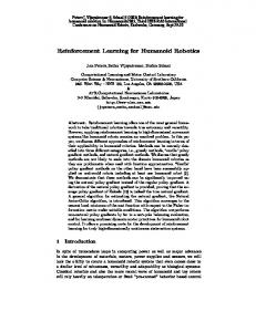
Initialize Q(s, a) arbitrarily ˜ s0 ← current system state; Choose a0 from π s ← s0 ; a ← a0 repeat ˜ Take action a; observe r and s′ ; choose a′ from π Q(s, a) ← Q(s, a) + η[r + γQ(s′ , a′ ) − Q(s, a)] s ← s′ ; a ← a′ until shutdown Fig. 1. The SARSA algorithm. Q(s, a) is the value function, π ˜ is the policy that selects a∗ = arg maxa Q(s, a) with probability 1 − ǫ and an arbitrary action a with probability ǫ, γ is the discount factor, and η is the learning rate.

is the action which maximizes the expected reward considering the current approximation Q (that is, a∗ = arg maxa Q(s, a)), then a∗ is selected with probability 1 − ǫ. To maintain a tradeoff between exploitation (using the knowledge gained so far) and exploration (looking for potentially better actions), with probability 1 − ǫ we select an action drawn randomly from among all the available actions. This is the so-called ǫ-greedy strategy where the parameter ǫ determines the explorationexploitation trade-off.

A. Markov decision process and reinforcement learning We first give the mathematical formalization of decision making. A Markov decision process (MDP) is a quadruple (S, A, P, R) where S is the set of possible states of the system, A is the set of actions (or decisions) that can be taken, and P is a collection of transition probabilities a ′ Pss ′ = P {st+1 = s |st = s, at = a}

that map the current state and action to the next state. The function a Rs,s ′ : S × A × S → R defines the rewards earned when moving from state s to state s′ through action a. The goal is to find a stationary policy π ∗ : S → A which chooses the action to take in each state, without knowledge of the past history (other than what is summarized in the state). The objective is to maximize the the long-term expectation of the rewards, the so-called value function "∞ # X π k γ rt+k+1 |st = s, at = a , Q (s, a) = Eπ

B. Grid scheduling and the reinforcement learning paradigm As explained before, a reinforcement learning formalization needs to define states, actions, and rewards for the given problem. A first contribution of our work is the proposition of a set of variables describing states and actions to allow the formulation of the grid scheduling problem as a continuous action-state space reinforcement learning problem. S TATE SPACE : THE GRID MODEL . A complete model of the grid would include a detailed description of each queue and of all the resources. This would be both inadequate to the MDP framework and unrealistic: the dimension of the state space would become very large. Instead, the state is represented by a limited set of real-valued variables. •

• •

•

k=0

where γ ∈ [0, 1] is a discount factor dampening the future rewards. In the scheduling context, P and R (the environment dynamics) are unknown, so the Q function has to approximated through repeated experiments. This is the definition of reinforcement learning [9]: the optimal policy will be learned by interactions with the environment. The general algorithm is an iterative process known as temporal-difference learning. The particular policy learning framework used in this work is based on SARSA, a classical reinforcement learning algorithm (fig. 1). SARSA is an on-policy learning algorithm: the approximate value function guides the selection of the current ˜ is action a, thus the reward r and the next state s′ . The policy π defined by the current approximation Q. More precisely, if a∗

•

the expected time remaining until any of the currently running jobs is completed; the number of currently idle machines; the workload (the total execution time of jobs waiting in the queues); the average user-utility (see below) expected to be received by the currently running jobs; the current share of resources resulting from previous allocation for each VO.

ACTION SPACE : THE JOB MODEL . Each waiting job is a potential action to be chosen by the scheduler. As a consequence, except if there is no job waiting, the scheduler will always select a job when a resource become available (greedy allocation). A job is represented by a set of descriptors (extracted for instance from the EGEE logging and bookkeeping system). The exact set of variables is under research, for the time being we are using 1) the type of the job (batch/interactive), 2) the VO of the user who submitted the job, and 3) the expected execution time, which is the time to complete the job without any queuing or management overhead. The first

two descriptors are actually available; the third one can be estimated from other descriptors. R EWARD : UTILITY FUNCTIONS . The overall utility of the scheduler is a combination of the time-utility, and the fairness. The time-utility function [3], [11], [12] is attached to each job, and it describes how “satisfied” the user will be if his/her job finishes after a certain time delay. It is typically a decreasing function of time, and it can vary with the job type. The fairness represents the difference between the actual resource allocation and the externally defined shares given to VO’s. These utility functions are described in more details in section IV-A. C. Continuous state-action space The state-action space is continuous (real valued). As a consequence, implementing the assignment Q(s, a) ← Q(s, a) + η[r + γQ(s′ , a′ ) − Q(s, a)] in fig. 1 is not immediate. The straightforward method would be to discretize the values (binning), and use a lookup table to represent Q(s, a). However, the space dimensionality is high: with 4 VO’s, the stateaction pace is R11 . The table representation would either require large bins (thus a very rough approximation) or a large number of bins that would result in excessively long training time. The alternative is to use a non-linear continuous approximation, as proposed in [10]. The design choice then lies in the interpolation method: one can use neural networks (NN), Gaussian processes [7]), or kernel methods, to cite a few of the available classes of algorithms. Because at this step there is no prior knowledge on the properties of the value function Q, similarly to [10], we opted for a neural net. Whatever method is used, the simple assignment in line 4. of the SARSA algorithm must be replaced by a learning procedure. In the case of the NN, there are two possibilities: stochastic on-line learning, where the network is modified in each iteration only using the newly acquired training example, and batch re-learning, where the NN is re-trained from scratch each time a new training example is added to the training set. For the time being we are using the batch option for simplicity. As pointed in [10], there are no theoretical guarantees that this combination of algorithms converges, however, in our experiments we did not have any problem with the convergence. The final ingredient in the definition of the algorithm is the initialization. In a very complex optimization landscape, running the modified SARSA algorithm with an untrained NN would lead to extremely bad decisions in the beginning. This would adversely impact the performance both because of the actual scheduling of the first jobs, and because of a poor initial approximation of the value function. To overcome this initialization issue, the RL system is trained off-line with an early deadline first policy. After a few learning sweeps using collected rewards, the network is quickly usable to take its own decisions and be optimized using real rewards. IV. T HE UTILITY MODEL A. Job utility functions Jensen at al. [3] introduced the concept of time utility functions (TUF). TUF’s provide a unified framework for

describing various QoS requirements including best effort, hard real-time, and soft real-time. In general, the TUF of a job is any function of time t which defines the user-perceived utility of completing a job at time t. In the most elementary setting, the TUF of a batch job is constant; the TUF of a hard real-time job is stepwise: up to the deadline L, the utility is constant and it becomes zero after the deadline. The TUF associated to soft-real time is constant up to the deadline and it decreases rapidly after. However, these simple utility functions 1) fail to capture the evident fact that a batch job must return in reasonable time, and 2) require a definition of deadline and a decreasing function for the real time jobs. In order to make a step towards selfconfiguration, the TUF should be derived in a semi-automatic fashion. We propose the following scheme for self-defined TUF (fig. 2). Let τj be the execution time of job j (here and in the following, job-related quantities are indexed by j in order to contrast them with the constants). •

•

•

•

The relative deadline dj (i.e., the absolute time deadline minus the submitting time aj ) is the execution time plus a fixed startup time σ: dj = τj + σ. Indeed, even extremely short jobs cannot expect to be completed instantaneously; σ captures the overhead associated with traversing the various middleware services before the job is dispatched on a site and starts waiting for available resources. The user should provide an indication of the QoS requirement associated to the job. In this work, we consider only a binary choice, between interactive and batch jobs. For batch jobs, the utility decreases over time following a power law with exponent β. For interactive jobs, the utility decreases exponentially over time at rate α.

Thus, we define the batch utility function UjB and the interactive utility function UjI as UjB (t) = UjI (t) = 1

if

aj ≤ t ≤ aj + dj ,

(1)

−α(t−aj −dj )

if

t > aj + dj ,

(2)

t − aj −β ) UjB (t) = ( dj

if

t > aj + dj .

(3)

UjI (t)

=e

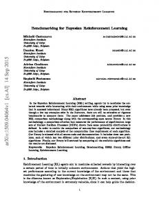
An important point is that these utility functions allow to define α and β in a way that is consistent with the high-level requirements of interactive and batch jobs. Consider u1/2 , the value of t for which the utility is 0.5 (half the maximal utility). In the interactive case, we get u1/2 = aj +dj +log(2)/α which shows that the user satisfaction depend on the wall-clock waiting time. In the batch case, the corresponding equation is u1/2 − aj = 2−β dj ; the penalty is roughly proportional to the execution time because the relative deadline dj is the execution time augmented by the overhead which should be negligible for batch jobs. Thus the shape of the utility curve for batch jobs scales with the job size while the shape of the utility curve for interactive jobs is fixed by external requirements. Within this framework, it is obviously possible to define multiple classes of service by varying the α and β parameters.

V. E XPERIMENTAL SETUP

1.2 interactive batch

time utility

1

A. The simulation platform

0.8 0.6 0.4 0.2 0 1

10

Fig. 2.

100 time

1000

10000

Self-defined time-utility functions

B. Fairness and productivity The allocation process should be such that the service received by each VO is proportional to some share. If there are n VO’s, the shares are usually expressed as a n-vector of the percentages of the total resources w = (w1 , . . . wn ). As stated before, these shares are a-priori parameters of the scheduling problem. Thus, contrary to the previous section, the modeling step should only address the following issue: define a function of the service actually received which is maximal when the proportionality is perfectly achieved. Let Sk (t) be the fraction of the total service received by VO k up to time t. Then, the deficit distance between the optimal allocation and the actual allocation is a good measure of the unfairness. The deficit distance is defined as D = max(wk − Sk )+ , k

where x+ = x if x > 0 and 0 otherwise. The unfairness is bounded above by M = maxk (wk ). A fairness utility can thus be derived by a simple linear transform. If M is the maximal unfairness, the fairness utility F is D F =− + 1. (4) M Some VO may ask for less than their share. Without greedy allocation, the previous rule leads to resource underutilization, a highly undesirable property. This classical problem has been addressed in the framework of network allocation as well as for processor allocation [5]) with the objective of fair excess allocation: if excess resources do exist, they should be proportionally allocated to the active requests. These methods could be adapted to our framework by dynamically adjusting the wk as a function of the actual requests. However, with greedy allocation, there is no risk of resource underutilization (as far as there is enough overall work). On the other hand, the excess resource can be advantageously exploited for favoring the user utility in the short term. Thus we keep the fairness utility as defined in eq. 4.

We developed a simulation framework for learning and evaluating grid scheduling policies. Our discrete event simulator supports multiple queues, fair-share measurement, multiple types of jobs, and independent definition of the scheduling policy. The RL scheduler uses the SARSA algorithm with NN training and the implementation of various utility functions. As a comparison baseline, we have also implemented a FIFO scheduler. Both the simulator and the schedulers are developed in MATLAB. In the reported experiments, we have used the following parameter values for the utility functions: α = 0.5, β = 0.3. With these values, the utility of an interactive jobs is down to 0.5 (i.e., half of the maximum utility) 1.3 units of time after the deadline, and the utility of a batch job is down to 0.5 when the turnaround time is approximately 10 times the execution time, meaning that the waiting time is 9 times the execution time. The startup time σ is 1 minute, which is consistent with experimental data on production grids. In the SARSA algorithm, the exploration-exploitation tradeoff parameter ǫ was set to 0.3, and the discount parameter γ was set to 0.2. The neural network is a standard multi-layer perceptron with one hidden layer containing 20 sigmoidal hidden units; the back-propagation learning rate is 0.3. B. The workloads We analyze two workloads. The first one is the traditional M/M/N queue, and the second one is extracted from real EGEE traces. The synthetic workload: The arrival process is Poisson with parameter λ and the execution times are exponentially distributed with parameter µ. The so-called utilization factor ρ = λ/µ must be less 1 in order to get a finite queuing time. The utilization factor controls the system load. In the following, ρ is set to 0.99. The system is thus heavily loaded which allows the RL algorithm to demonstrate its superior performance. Interactive jobs are defined to be jobs with an execution time less than 15 min. The proportion of interactive jobs varies across the experiments. The value of µ follows immediately from the definition of the exponential distribution P (X > t) = e−µt . For a given ρ, λ is then computed as µρP , where P is the number of processors. In this experiment, P is set to 50. For all the experiments, 6000 jobs are simulated. The last 500 jobs are not taken into account in the reported results in order to avoid the experimental bias due to the period where the queue is draining. Table I gives the resulting configurations. In the experiments, we compare the performance of our method with a baseline FIFO scheduling. The same input files (created using the parameters described in TableI) are used for both methods. The EGEE workload: This experiment uses traces of real EGEE jobs as input. The trace covers the activity of more than one week (17-26 May 2006) at the LAL site. It includes 6000

0.2 0.4 0.5

µ

2.48E-04 5.68E-04 7.70E-04

λ

1.23E-02 2.81E-02 3.81E-02

Mean exec. time (minutes) 67 29 22

Simulated duration (hours) 136 59 44

TABLE I S YNTHETIC WORKLOAD CONFIGURATIONS .

1

0.99

0.98 Fairshare reward

Exp.

0.97 RL FIFO

0.96

0.95

0.94

0.93

0

0.5

1

1.5

2

2.5 Time

user jobs, not counting the monitoring jobs which are executed concurrently with the users jobs and consume virtually no resource; they were removed from the trace. In this period, the number of processors is fairly constant (P = 100). The site has been restructured many times in the whole extent of the trace, increasing its resources from 25 to 400 processors. The jobs with execution time less than 15 minutes are considered interactive: these jobs form more than 62% of the total number of jobs but less than 3% of the workload. The native site scheduler is MAUI/PBS with the SDJ mechanism enabled. The bound for the execution time of such jobs was 15 minutes. Thus, in the applied workload, jobs of less than 15 minutes can be either SDJ jobs or batch jobs depending on the user request. C. Performance metrics The first question is the execution time of the RL algorithm itself, that is, the time to take a scheduling decision. Within our MATLAB platform, the average execution time of the RL algorithm ranges from 1 to 10 ms, depending on the load. Indeed, the RL scheduler has to scan the waiting jobs in order to select the one maximizing the reward, so the execution time depends on the system load. Obviously, a real-world scheduler would not be implemented in MATLAB; our point here is to demonstrate that the RL scheduler is realistic. The most important performance indicators are related to the satisfaction of the grid actors. From the user’s point of view, we consider two indicators. The first one is simply the wallclock waiting time. The second one is the relative overhead which is the ratio of the waiting time to the execution time. Considering fair-share, we report the instantaneous reward which is the linear function of the distance to the optimum presented in equation 4. VI. P ERFORMANCE RESULTS A. The synthetic workload: feasible schedule In this experiment, we have 4 VO’s with with fair-share target weights 0.7, 0.2, 0.05, and 0.05. The schedule is feasible, meaning that the actual work proportions in the overall synthetic workload are the same as the target weights. In addition, inside each class of jobs (interactive and batch), the proportions are also close to the target. The statistics of the waiting times are summarized in table II. The first column gives the fraction of interactive jobs in the workload.

Fig. 4.

3

3.5

4

4.5 5

x 10

Dynamics of the fair-share.

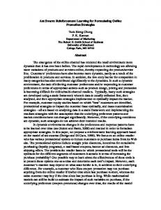
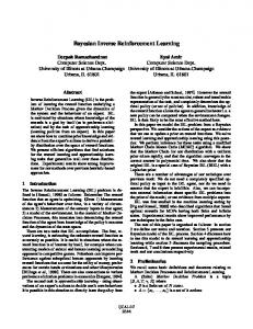
These results indicate that the RL-method clearly outperforms FIFO: the delay is divided by more than 8 when there are 20% of interactive jobs, and by nearly 20 at 50%. This improvement holds with similar values for both the interactive class and the batch class. One can suspect that favoring interactive jobs results in nearly starving some batch jobs, however, the reduced standard deviation and maximum indicate that this is not the case. The cumulative distribution function of the waiting time is shown on fig. 3 (left graph) for the interactive class. An important result is that the delay becomes acceptable for human interaction: in the worst case (20% of interactive jobs) 90% do not wait more than 2 minutes. The cumulative distribution function of the relative overhead for the interactive class is shown on fig.3 (right graph). In summary, the waiting time is at most equal to the execution time for 90% of the jobs with RL, while this is true only for 30% of the jobs with FIFO. Fig. 5 shows an example of the dynamics of the fair-share performance: the horizontal axis is the simulated time and the vertical axis is the fair-share utility. The first 500 jobs are skipped in order to make the figures readable (with the initial small sample, both have very poor performance so the vertical range is too large). With a feasible schedule, in the long run, the job sample agrees with the target, thus the FIFO scheduler achieves the requested fair-share. The RL-method is slightly inferior to FIFO in the long run. However, the price to pay is extremely small: in both cases the RL method is only 3% off the ideal allocation. In addition, the RL method converges reasonably fast considering the grid time scale: at time 50000 (13 hours), the fair-share utility is above 94%. The figures for the other cases (40% and 50% of interactive jobs) are quite similar so we omitted them. B. The synthetic workload: infeasible schedule The “high level” objectives defined by humans may be unrealistic. It is well known that this is often the case for fair-share. The target weights describe the activity of users as expected by administrators, and they may significantly differ from the actual activity. In this experiment, we consider the case where the target weights are 0.4, 0.2, 0.2, and 0.2, while the actual weights remain 0.7, 0.2, 0.05 and 0.05.

Exp. 0.2 0.4 0.5

FIFO-Inter mean std max 923 552 2361 690 321 1425 740 368 1577

mean 108 50 38

RL-inter std 123 58 42

max 975 597 368

FIFO-batch mean std max 825 539 2383 642 314 1426 718 360 1550

mean 103 454 343

RL-batch std 112 49 38

max 1040 515 397

TABLE II WAITING TIME FOR THE SYNTHETIC WORKLOAD WITH A FEASIBLE SCHEDULE . A LL TIMES ARE IN SECONDS .

1

1 fifo20 RL20 fifo40 RL40 fifo50 RL50

0.9

0.8

0.7

0.7

0.6

0.6 cdf

cdf

0.8

0.5

0.5

0.4

0.4

0.3

0.3

0.2

0.2

0.1

0.1

0 1e+00

1e+01

1e+02

1e+03

fifo20 RL20 fifo40 RL40 fifo50 RL50

0.9

1e+04

0 1.0e-03

1.0e-02

time (sec)

Fig. 3.

1.0e-01

1.0e+00

1.0e+01

1.0e+02

1.0e+03

1.0e+04

overhead

Performance comparison for the feasible schedule under RL and under FIFO.

This is an infeasible schedule because the first VO does not provide enough load, and the third and fourth VO’s ask for more resources than they are entitled to. Nonetheless, the overall load remains compatible with the resources: the preset utilization factor is the same 0.99 as before. The dataset is the same as in the previous experiment; only the weight parameters in the fair-share utility function are modified. The issue here is to assess the robustness of our RL-method in presence of infeasible constraints. According to eq. 4, the maximal positive distance is 0.2−0.05 = 0.015, and the upper bound for unfairness is 0.4, thus the best possible schedule gives a reward of 0.625. Fig. 5 show sthat the RL and FIFO achieve comparable and nearly optimal performance in this challenging case. The results on user related metrics are very similar to the feasible case, thus we do not repeat them. C. The EGEE workload The distribution of the workload is much more complicated than in the synthetic case. The workload is heavily dominated by short jobs. The workload is heavily dominated by short jobs which is a general feature of a significant part of the EGEE workload [2]. As explained in section II-B, the accepted SDJ jobs are executed immediately, within reserved slots. More precisely, they are executed concurrently with batch jobs using time sharing. It follows that the goal of the RL algorithm is different from the goal in the synthetic cases: by construction, SDJ jobs have a very small waiting time and a very small overhead, thus the native scheduler cannot be outperformed on these jobs. The challenge for the RL algorithm is to provide acceptable results for all interactive jobs (SDJ and non-SDJ) without prior

Mean Median Max Std

Native-Inter 5876 531 52692 10226

RL-Inter 2163 352 20118 3914

Native-Batch 7695 3214 55376 10619

RL-Batch 1717 200 22947 3482

TABLE III WAITING TIME FOR THE EGEE WORKLOAD . A LL TIMES ARE IN SECONDS .

reservation and time-sharing. As time-sharing raises objections from some users and administrators in the EGEE community, exploring alternative mechanisms is a practical issue. The statistics of the waiting times are summarized in table III. The standard deviation being much larger than the mean, we also report the median. For interactive jobs, RL outperforms the native scheduler by more than two-fold on all quantities. For batch jobs, the result is even more impressive: the median waiting time is lowered by more than an order of magnitude. Fig. 6 gives a detailed comparison of the performance of the native and the RL-scheduler. The left graph shows the cumulative distribution function of the waiting time. For interactive jobs, the RL-scheduler obtains a reasonable waiting time (less than 2 minutes) for only 40% of the jobs, and is only marginally better than the native scheduler after that. The problem here is the learning period. The right graph in fig. 6 shows the dynamics of the waiting time. More precisely, the graph plots the difference between the waiting time under the native scheduler and under RL as a function of arrival date. After approximately half of the jobs, the RL-scheduler

0.67

0.65 fifo20 RL20

0.66

fifo50 RL50 0.64

0.65 0.63 0.64 0.62 FS

FS

0.63 0.62 0.61

0.61 0.6

0.6 0.59 0.59 0.58

0.58 0.57

0.57 5e+04

1e+05

2e+05

2e+05

2e+05

3e+05

4e+05

4e+05

2e+04

4e+04

6e+04

time (sec)

8e+04

1e+05

1e+05

1e+05

time (sec)

Fig. 5.

Dynamics of the fair-share with infeasible schedule. 6E+04

1

5E+04

0.9

4E+04

0.8

3E+04 0.7 2E+04 time(s)

cdf

0.6 0.5

1E+04 0E+00

0.4 -1E+04 0.3

-2E+04

0.2

-3E+04

Maui-int RL-int Maui-batch RL-batch

0.1 0 1e+00

1e+01

1e+02 1e+03 time (sec)

1e+04

-4E+04 1e+05

-5E+04 0E+00

1E+05

2E+05

3E+05 4E+05 5E+05 arrival date (s)

6E+05

7E+05

8E+05

Fig. 6. Performance comparison for the EGEE workload under RL and under the native scheduler. Left graph: Cumulative distribution function of the waiting time. Right graph: WaitingTimenative − WaitingTimeRL .

scheduler and the native scheduler. The RL scheduler achieves nearly the same performance, the difference being constantly below 0.01.

1e-02

Diff. fair-share

8e-03 6e-03 4e-03

VII. C ONCLUSION

2e-03 0e+00 -2e-03 -4e-03 -6e-03 0e+00

Fig. 7.

2e+05

4e+05 time (sec)

6e+05

Difference in fair-share under RL and the real scheduler

behaves consistently better than the native scheduler and it is continuously improving. Thus, the RL method is in fact able to outperform the native scheduler, however, the learning phase is much longer than in the synthetic case. In the conclusion we will outline the path to speedup the learning phase. Figure 7 shows the difference in the fair-share under the RL

The main contribution of this paper is the presentation of a general scheduling framework for providing both QoS and fair-share in an autonomic fashion, based on 1) configurable utility functions and 2) RL as a model-free policy enactor. Combining RL methods and utility functions for resource allocation has been pioneered by Tesauro [11], [10], Vengerov [12], and Whiteson and Stone [13]. Tesauro’s work targets optimal allocation of resources for Data Centers, thus optimizes the fraction of a global pool allocated to each application, while we are seeking an optimal schedule. Nevertheless, the resource allocation issues are very similar. The main difference in our work is that we consider a multicriteria optimization problem, including a fair-share objective. The main contribution of Whiteson and Stone was to use genetic programming for neural network parameterization in the context of Q-learning. They demonstrated their method on a simplified job server scheduling application with 100 jobs,

4 types of utility functions, and a unique reward function as a sum of individual utility functions. The comparison with a real and sophisticated scheduler shows that we could improve the most our RL scheme by accelerating the learning phase. More sophisticated interpolation (or regression) could speedup this phase. We plan to explore a hybrid scheme [10], where the RL is calibrated off-line by using the results of a real scheduler. Acknowledgments This work has been partially supported by the EGEE-II project funded by the European Union INFSO-RI-031688. R EFERENCES [1] F. Gagliardi et. al. Building an Infrastructure for scientific Grid computing: status and goals of the EGEE project. Philosophical Transactions of the Royal Society A, 1833, 2005. [2] C. Germain-Renaud, C. Loomis, J.T. Mo’scicki, and R. Texier. Scheduling for responsive grids. Journal of Grid Computing, 2007. on line doi= 10.1007/s10723-007-9086-4. [3] E. Douglas Jensen, C. Douglas Locke, and Hideyuki Tokuda. A timedriven scheduling model for real-time operating systems. In IEEE RealTime Systems Symposium, pages 112–122, 1985. [4] Jeffrey O. Kephart and David M. Chess. The vision of autonomic computing. IEEE Computer, 36(1):41–50, 2003. [5] L.Amar, A. Barak, E. Levy, and M. Okun. An on-line algorithm for fairshare node allocations in a cluster. In CCGRID, pages 83–91, 2007. [6] I. Mirman. Going Parallel the New Way. Desktop Computing, 10(11), June 2006. [7] Carl Edward Rasmusen and Chris Williams. Gaussian Processes for Machine Learning. MIT Press, 2006. [8] Lawrence G. Roberts. Beyond moore’s law: Internet growth trends. Computer, 33(1):117–119, 2000. [9] Richard S. Sutton and Andrew G. Barto. Reinforcement Learning: An Introduction. MIT Press, 1998. [10] Gerald Tesauro, Nicholas K. Jong, Rajarshi Das, and Mohamed N. Bennani. On the use of hybrid reinforcement learning for autonomic resource allocation. Cluster Computing, 10(3):287–299, 2007. [11] Gerald J. Tesauro and Jeffrey O. Kephart. Utility functions in autonomic systems. In Proceedings of the 1st International Conference on Autonomic Computing(ICAC’04), pages 70–77, 2004. [12] D. Vengerov. A reinforcement learning approach to dynamic resource allocation. Eng. Appl. Artif. Intell., 20(3), 2007. [13] S. Whiteson and P. Stone. Evolutionary function approximation for reinforcement learning. Journal of Machine Learning Research, 7:877– 917, 2006.