a priori segmentation of the highway system is also explored. Longer, ... improvements can be divided into three types; before-after studies, cross- sectional ...
Environmental Health Risk IV
85
Validation and implication of segmentation on Empirical Bayes for highway safety studies R. R. Souleyrette, R. P. Haas & T. H. Maze Iowa State University, SAIC and Iowa State University, USA
Abstract Typically, crash frequency is modelled as Poison where the variation is the square root of the expected number. If the expected number of crashes is small, the variation is a large percentage of the expected number of crashes, and the observed number of crashes provides a crude estimate for the expected number. A better estimate is obtained when the expected number is large. For a specific location, there are two approaches for performing measurements where the expected number of crashes is large. One approach is to measure over a long period of time. However, data are not often available for long periods. Even if available, changes in conditions over time, such as increase in traffic volumes or improvement in infrastructure, may limit the useful time frame. Another approach is to perform measurements over a large number of similar locations, providing a relatively precise estimate for the distribution. Then, one can use the Empirical Bayes (EB) approach to combine the relatively precise estimate for the distribution with the less precise estimate for the expected number at the location of interest, resulting is an improved estimate for the expected number at that location. This paper explores the two approaches. It uses multiple years of data from the Highway Safety Information System for California intersections and highway links from the State of Iowa. Data from a single year is used to estimate the expected number of crashes at locations, following the EB approach. Data from multiple years at each location is then used to estimate the expected number of crashes at those locations, and the results from the two approaches are compared. No such large scale validation has yet been performed. The effect of a priori segmentation of the highway system is also explored. Longer, homogeneous sections are found both to improve the statistical validity of models and to improve the EB correction of one-year section crash estimates. Keywords: count models, Empirical Bayes, crash frequency estimations, segmentation for crash sampling. WIT Transactions on Biomedicine and Health, Vol 11, © 2007 WIT Press www.witpress.com, ISSN 1743-3525 (on-line) doi:10.2495/EHR070101
86 Environmental Health Risk IV
1
Introduction
The traditional methods for determining the benefit of roadway safety improvements can be divided into three types; before-after studies, crosssectional studies, and regression studies. By far the most commonly used technique is before and after studies where one physical change is made to a location or locations and the analyst waits to see if crash trends at the location(s) are improved. The problem with this method is that it requires data for several years before and after the change and does not take into account temporal changes that occur in the after period (changes in stream composition, changes in automobile design, climate changes, etc.) Another traditional method is to use cross-sectional studies where one group of similar locations is treated with and another group of similar locations are not treated (sometimes called case/control studies). The problems with cross-sectional studies are that they ignore spatial differences (e.g., changes in land use, changes in traffic volumes, changes in enforcement policies, etc.) and place the safety engineer in the moral dilemma of specifically not applying a treatment to a control group where the engineer may believe the changes will improve safety. To increase the number of data cases, cross-sectional data can be combined with case/control data, however, controlling for similarities in intersection geometry and volume is particularly critical. Often time there are a small number of very similar sites or a large number of sites with variations (traffic volume and geometry) which compromise the comparison. Another common method is to model crash performance, typically using Poisson or Negative Binominal regression (commonly called a count model) to create Safety Performance Functions (SPFs). SPFs commonly include traffic volumes, traffic characteristics and patterns (e.g., percent trucks) and geometric differences in the highway. The regression model cannot take into account every variable that is responsible for a crash and there is a good deal of multi colinearity between variables. As a result, typically regression models account for only a minority of the variance in crash counts and making them relatively inaccurate when it comes to estimating the benefits of a treatment. The Empirical Bayes (EB) approach combines the strengths of before-after studies, cross-sectional studies, and regression methods when estimating the safety related benefits of an improvement. EB uses data from a group of similar control sites and pre-treatment data from the case site to determine the crash performance before the improvement is made. This allows comparison of the after treatment safety performance at a site to estimate the expected safety performance had the improvement not been made. The difference during this period is the “safety benefit” of the treatment. In other words, EB bases the expected safety performance (without the treatment at the site) on the performance observed at the site prior to treatment, and the performance at similar sites. EB reduces the variability of estimates of safety performance beyond traditional methods. (1) EB also helps to diminish the impact of regression to the mean. Regression to the mean impacts estimates when treatments are applied to roadway segments or WIT Transactions on Biomedicine and Health, Vol 11, © 2007 WIT Press www.witpress.com, ISSN 1743-3525 (on-line)
Environmental Health Risk IV
87
intersections that may be randomly experiencing poor safety performance. Even without the treatment, the safety performance is likely to improve. Because EB estimates rely on untreated locations, use of a safety performance sample from similar untreated sites tends to reduce the impact of regression to the mean.
2
Overview of Empirical Bayes
One of the challenges in working with traffic crash statistics is generating accurate estimates for the expected number of crashes per year at a location. The root of the difficulty is that the actual number of crashes follows a Poisson distribution with mean (λ) equal to the expected number of crashes, and this distribution is broad for the types of locations typically studied in transportation. As a rough estimate, the 95% confidence interval for λ is
λ±2 λN
, where N
is the number of years for which data are available. For a location where the expected number of crashes is 20, the 95% confidence interval has width 18 for a single year of crash data. A single year of data provides a very unreliable estimate for the expected number of crashes. One way to improve the estimate for the expected number of crashes is to use multiple years of crash data. For five years of crash data, the width of the 95% confidence interval is 8. For ten years of crash data, the width is about 5.6. It is not practical to use longer periods because traffic conditions are likely to have changed so much over such long periods that the historical crashes are no longer good indicators of the number of crashes that would currently occur. An alternate method for providing more accurate estimates for the expected number of crashes, would be to group together data from a large number of identical locations. Since the locations are identical, the expected number of crashes at each location would be the same, and the observations from these locations can be combined to estimate λ. In essence, one replaces a long timeseries of crash data at a single location with crash data from a large number of identical locations. While this is a good approach in theory, in the real world, there are no “identical locations”. In the real world, the expected number of crashes for a collection of similar locations will be close to each other, but not exactly the same. The Empirical Bayes approach takes this into consideration by combining the distribution in the observed number of crashes that comes about because of the Poisson nature of crashes with the distribution for the expected number of crashes at similar locations. The Empirical Bayesian formula is:
ϕ n 1 Nλ0 λ = λ0 + N 1+ ϕ 1+ ϕ Nλ0 Nλ0 where λ0 is the average number of crashes per year for the entire collection of locations, n is the number of crashes observed at the location of interest during N WIT Transactions on Biomedicine and Health, Vol 11, © 2007 WIT Press www.witpress.com, ISSN 1743-3525 (on-line)
88 Environmental Health Risk IV years of observations, and φ is a parameter that indicates how much variation exists in the expected number of crashes for the locations in the collection. If φ is large, the variation in the expected number of crashes is small; if φ is small, the variation is large. One can see this in the formula above. If φ is large, the expected number of crashes is close to λ0 for all the locations in the collection, so the formula weights the λ0 term more strongly. If φ is small, the opposite occurs. One can think of the collection of similar locations as providing a model for the location of interest. Thought of in this way, the Empirical Bayes formula generates an improved estimate for the expected number of crashes for a location by taking a weighted average of an estimate based on crash data for that location and an estimate based on the model. The value for the weight changes to place more emphasis on the more accurate of the two approaches. This thought process points to another way to improve estimates for the expected number of crashes. In the above formula, the simplest model was used to estimate the expected number of crashes for locations in the collection – the average for the collection. One could further improve the estimate for the expected number of crashes at the location of interest by using a better model for the expected number of crashes in the collection. An improved model will result in lower unexplained variance in the collection, a higher value for φ, and greater weight for the model term in the Empirical Bayesian formula. Because the EB formula places more weight on the more accurate model, the resulting estimates for the expected number of crashes at the location of interest should be more accurate.
3
Research objective
The objective of this research is to explore the relationship between the effectiveness of the Empirical Bayesian formula at correcting estimates for the expected number of crashes at a location and the accuracy of the model for the expected number of crashes in the comparison group. To meet this objective, crash data were collected for both a large number of similar locations and for a number of years at each location. Comparisons were made between estimates for the expected number of crashes using, 1) a single year of data with different models and the Empirical Bayesian formula, and 2) several years of crash data at specific locations. These comparisons verify the value of the Empirical Bayesian approach at improving estimates for the expected number of crashes and emphasize the importance of an accurate model for the expected number of crashes in the comparison group. A second objective is to explore the relationship between segmentation and accuracy of estimates, as crash data must be aggregated to units of analysis prior to processing.
4
Description of the data used
Two types of data were used for this research. The first type of data was crash data and road inventory data from Iowa. Both the crash and road inventory data are maintained by the Iowa Department of Transportation (a USA state level WIT Transactions on Biomedicine and Health, Vol 11, © 2007 WIT Press www.witpress.com, ISSN 1743-3525 (on-line)
Environmental Health Risk IV
89
agency) and are available to support safety analysts. For this analysis, five years of crash data were compiled for more than 7,000 miles of Iowa roads. The roads were classified into three primary categories: 2-lane roads, multi-lane and divided roads, and freeways and Interstates. The 2-lane roads were further subdivided into low, medium, and high volume roads based on average annual daily traffic (AADT). To support this research, the roads were divided into segments. Analysis was conducted on the annual number of crashes for these segments. Three different sizes of segments were used: short segments with approximate length of 0.25 miles, medium segments with approximate length of 2.5 miles, and long segments with approximate length of 4 miles. All in all, this created fifteen collections of segments for which crash models were developed. The second type of data was crash and road inventory data from the US Federal Highway Administration, Highway Safety Information System (HSIS). The HSIS data are collected from seven participating States and maintained by the Federal Highway Administration to support highway safety research. (More information is available from the HSIS website at http://www.hsisinfo.org/.) For this research, five years of crash and road inventory data were provided for the approximately 18,000 junctions (intersections) included in the California HSIS data. One limitation regarding the California HSIS data was noted – few of the cross street volumes had been recently updated. The data were filtered to identify intersections for which key intersection attributes (i.e., intersection geometry and type of traffic control) were constant over the five-year period and the number of crashes per year was tallied for each of these intersections. As with the Iowa data, the intersections were then divided into groups based on the intersection geometry and the type of traffic control at the intersection, and crash models were developed for the different groups of intersections. This resulted in three datasets: multi-phase signal control (873 intersections), single-phase signal control (374 intersections) and two-way stop-control, aka through-stop control (3047 intersections).
5
Analysis approach
For each of the 15 road section datasets and for the three intersection datasets, negative binomial safety performance functions (SPFs) were fit using the R program (available at http://www.r-project.org/) While five years of crash data were available, only 2004 crash data were used to develop the models. This was to demonstrate the use of EB where several years of crash data may not be available. Road models (SPFs) are of the general form: Crashes = α Length (AADT)β. Table 1 presents the road model parameters and descriptive statistics. The intersection model (SPF) are of three forms: a) Crashes = α(ADTML)β, b) Crashes = α(ADTML)β(ADTXS)γ, or c) Crashes = α (ADTML)β(NXSL)δ, where ADTML is average daily traffic on the main line, ADTXS is ADT on the cross street and NXSL is the number of cross street lanes. Table 2 presents the intersection model parameters and descriptive statistics.
WIT Transactions on Biomedicine and Health, Vol 11, © 2007 WIT Press www.witpress.com, ISSN 1743-3525 (on-line)
90 Environmental Health Risk IV
Avg. length
Avg AADT
0.28 0.23 0.13 0.32
5614 16315 8714 2689
road type
# segments
Road model parameters and descriptive statistics.
19536 3684 4228 19459
Segment Length
ID
Table 1:
all Freeway multi-divided 2-lane 2-lane 6493 0.37 1225 low AADT 5 2-lane 6491 0.34 2398 med AADT 6 2-lane 6478 0.26 4440 high AADT 7 2983 2.59 4785 All 8 364 2.36 16166 Freeway 9 276 1.98 7963 multi-divided 10 2343 2.7 2643 2-lane 11 1508 5.1 4185 All 12 119 7.23 1574 Freeway 13 153 3.65 8324 multi-divided 14 1236 5.08 2605 2-lane 15 * model parameter is not statistically significant.
α 0.0034 0.0022 0.0019 0.0013
β 0.7281 0.7453 0.8327 0.8497
φ 1.20 1.82 0.71 1.17
0.6038*
-0.0106*
0.93
0.0030
0.7228
1.36
0.0000 0.0029 0.0020 0.0023 0.0013 0.0020 0.0008 0.0023 0.0014
1.4368 0.7433 0.7583 0.7968 0.8442 0.7904 0.8555 0.7955 0.8334
1.22 3.01 3.88 5.43 2.86 3.42 3.74 7.09 3.24
Long
Med
Short
1 2 3 4
Number of intersections
Avg ADTML
Avg ADTXS
Avg NXSL
873
31388
7775
2.804
374
3047
Model Form
Control type
Multip hase signal Single Phase signal
Intersection model parameters and descriptive statistics.
Thrustop
Table 2:
2.5695
1.9829
6251
789
14086
28413
Į a 0.067 b 0.047 c 0.081 a 0.059 b 0.018 c 0.053 a 0.002 b 0.002 c 0.002 * model parameter is not statistically significant.
ȕ 0.427 0.363 0.388 0.429 0.411 0.419 0.684 0.515 0.687
WIT Transactions on Biomedicine and Health, Vol 11, © 2007 WIT Press www.witpress.com, ISSN 1743-3525 (on-line)
Ȗ
į
0.120 0.224 0.164 0.238* 0.303 -0.144*
ij 1.649 1.727 1.669 1.330 1.408 1.340 0.896 1.080 0.897
Environmental Health Risk IV
Figure 1:
91
Example road SPFs.
Most of the models fit produced statistically valid results. Exceptions were the low volume 2-lane model and two of the intersection models based on cross street number of lanes as a proxy for cross street ADT (as confidence in the cross street ADT values was low, models were also fit on NXSL as a proxy). Figure 1 illustrates freeway and AADT variant 2-lane models derived from the various levels of segmentation used in this research.
6
Analysis results
To illustrate the effects of segmentation and choice of “comparable data” on the results of the EB procedure, several “high crash” road segments and intersections were selected. These locations were chosen based only on their 2004 crash experience. The purpose was to compare EB estimates for these high crash locations to their five-year crash performance average and to demonstrate the effect of various levels of data aggregation. Recall that data aggregation was performed across two dimensions, segment length (short, medium and long) and similarity of segments (road type, intersection control, AADT class, etc.) A total of nine road sections, all of the freeway/Interstate class, were selected as “high crash locations.” Three each were selected from each of the three road segmentation databases (low, medium and high). Table 3 presents the comparison of EB estimate to five-year average crash frequencies. It can be seen that the EB correction is most accurate when longer segmentation is used. While the shortest segmentation provides the greatest homogeneity, the longer sections values are corrected most closely to their five-year averages. Three intersections, all of the multi-phase signalized class, were also selected as “high crash locations.” Table 4 presents the comparison of EB estimate to five-year average crash frequencies. It can be seen that the EB provides very good adjustments to the single year crash numbers – placing the expected value much closer to the five-year average. (Recall that only one year of data was used to derive the EB corrected estimates.) WIT Transactions on Biomedicine and Health, Vol 11, © 2007 WIT Press www.witpress.com, ISSN 1743-3525 (on-line)
92 Environmental Health Risk IV
short
med
long
Length 0.35 0.46 0.24 1.01 0.86 0.65 1.88 0.65 3.56
Crashes in 2004
EB estimate
c
XSTLANES
b
Intersection case studies.
XSTAADT
a
Crashes 5yr avg in 2004 Model EB estimate crashes 3.69 6 5.63 2.0 2.87 7 6.18 5.4 1.77 8 6.22 4.8 5.79 16 11.9 10.2 5.30 23 15.5 19.8 3.11 26 13.3 15.0 8.53 25 20.0 21.6 3.51 26 14.4 15.0 12.75 35 30.0 25.4
ML_AADT
model
Table 4:
AADT 30600 16300 19900 35444 38953 27948 22828 27948 17312
22750 18700 24000 22750 18700 24000 22750 18700 24000
3300 27200 4750 3300 27200 4750 3300 27200 4750
2 4 4 2 4 4 2 4 4
23 21 20 23 21 20 23 21 20
18.4 16.4 16.2 18.1 17.4 16.1 18.1 17.0 16.6
1.649
1.727
1.669
5yr average crashes
Segmentation
Road section case studies.
φ
Table 3:
14.6 15.8 12.4 14.6 15.8 12.4 14.6 15.8 12.4
A more detailed comparison was also conducted across all of the intersections. In this comparison, the standard deviation of the difference between the number of crashes in 2004 and the 5-year average was 2.43. For model a, the standard deviation was 3.95. When the EB formula was used to combine the model with the 2004 observations, the standard deviation was 2.03. In other words, the model by itself provided a poor estimate for the expected number of crashes, but improved the estimates when used with EB and a single year of crash data.
WIT Transactions on Biomedicine and Health, Vol 11, © 2007 WIT Press www.witpress.com, ISSN 1743-3525 (on-line)
Environmental Health Risk IV
7
93
Conclusions
This paper demonstrates the effectiveness of EB at improving estimates for the expected number of crashes for road segments and intersections. For road segments, a simple model was applied to fifteen different road segment databases. A sample of nine segments was considered and comparisons made between the 5-year average number of crashes for these segments and the estimates of the expected number of crashes based on a single year of data at that location, a model for crashes at similar locations, and the EB combination of the two. These examples demonstrate how EB improves estimates over use of either a single year of data or the model alone. These examples demonstrate another feature related how the explanatory power of the model impacts the effectiveness of EB. Table 1 indicates that the term φ is significantly lower for short segments than for medium and long segments. This indicates that, for short segments, there is greater variability about the model estimates than for longer segments. In other words, the model is a better estimator of the expected number of crashes for medium and long segments. The EB formula takes this into consideration when adjusting the estimate for the expected number of crashes. For medium and long segments, the model is more accurate. Because of this, the EB formula places a higher weight on the model, increasing the overall effect of the model on the EB estimate. This is apparent in Table 3 because the EB adjustment for short segments is very small (because φ indicates that the model is not very accurate) and the EB adjustment for medium and long segments is much larger. For intersections, several different models were developed for three different types of intersections. Table 4 lists the model and EB estimates for 3 example intersections. Even though the differences in φ are small, larger values of φ still correspond to better EB estimates for the 5-year average of the number of observed crashes. A comparison of the single-year, model, and EB estimates for the expected number of crashes for all the intersections with multi-phase signal controllers provides further evidence of the power of EB. EB combined two estimates for the number of crashes at each intersection, one with a root-mean square difference of 2.43 from the average of 5-years of observations and one with a root-mean square difference of 3.95, to produce an EB estimate with rootmean square difference of 2.03. Thus, EB combined two relatively poor estimates for the expected number of crashes at these intersections to produce a significantly improved estimate. These results demonstrate how EB improves estimates for the expected number of crashes for road segments and at intersections. For the intersections in this study, the use of EB with very simple model resulted in a 20% improvement in estimates for the expected number of crashes at these intersections. Better results would be expected with a more accurate model. The road segment results listed in this paper provide some support for this statement. The improvement in estimates for short segments (where φ was small, indicating more variance unexplained by the model) was less dramatic than for medium and long segments (where φ was larger and there was less unexplained variance). WIT Transactions on Biomedicine and Health, Vol 11, © 2007 WIT Press www.witpress.com, ISSN 1743-3525 (on-line)
94 Environmental Health Risk IV
References [1] Hauer, E.; Harwood, D.; Council, F.; Griffith, M.; “Estimating Safety by the Empirical Bayes Method: A Tutorial”. Transportation Research Record No. 1784, Statistical Methodology: Applications to Design, Data Analysis, and Evaluation. 2002. pp. 126-131.
WIT Transactions on Biomedicine and Health, Vol 11, © 2007 WIT Press www.witpress.com, ISSN 1743-3525 (on-line)