Author manuscript, published in "Acustica 90 (2004) 731-745"
F. Treyssède, Acustica
Validation of a finite element method for sound propagation and vibro-acoustic problems with swirling flows
Fabien Treyssèdea), and Mabrouk Ben Tahar Université de Technologie de Compiègne, Laboratoire Roberval UMR 6066,
hal-01064471, version 1 - 16 Sep 2014
Secteur Acoustique, BP 20529, 60205 Compiègne Cedex, FRANCE
Received: Suggested running title: “A FEM model for sound propagation in swirling flows”
a)
Electronic mail:
[email protected]
1
F. Treyssède, Acustica
Abstract: The goal of this paper is to propose a general finite element method (FEM) for sound propagation and vibro-acoustic problems in the presence of swirling ducted flows. The numerical method has already been successfully tested for sheared flows in the authors’ recent papers. The acoustic variational formulation is based on a non-standard wave equation established by Galbrun in 1931, which describes exactly the same physical hal-01064471, version 1 - 16 Sep 2014
phenomenon that the linearized Euler’s equations (LEE). Though this equation is only written in terms of the Lagrangian perturbation of the displacement, a mixed pressuredisplacement formulation is preferred in order to avoid a locking phenomenon. Furthermore, the coupling conditions for vibro-acoustic problems are naturally introduced. The FEM method proposed in this paper is compared in the axisymmetric case to a semi-analytical model, which is a generalisation of Pridmore-Brown equation to a duct with swirling flows and vibrating walls. A first set of results is compared with semi-analytical solutions for a rigid wall duct. A second set of results concerns the vibroacoustic interactions of a straight duct with an elastic outer wall.
PACS numbers: 43.20.Bi, 43.28.Py, 43.20.Mv, 43.20.Tb
2
F. Treyssède, Acustica
I.
INTRODUCTION
Propagation of acoustic disturbances in a swirling duct flow is a subject of considerable interest in many industrial applications, particularly when turbomachines are involved. For instance in aeroengine ducts, rotating fans generate a significant
hal-01064471, version 1 - 16 Sep 2014
swirling flow that may affect the propagation of sound. The mainly used basic equations that describe such a problem are the linearised Euler’ s equations (LEE). The scalar fullpotential equation, which is very often used for sound propagation in moving flows thanks to its simplicity1,2,3,4, cannot be considered here because of the flow rotationality.
Kerrebrock5 was one of the first to study the disturbances that propagate in a mean flow swirl, typically happening behind a rotor stage. Based on the LEE, he derived and solved a scalar equation in the particular case of a mode propagating in a straight duct. Roger and Arbey6,7 also analysed pressure waves in pipes with swirling flows.
More recently, Golubev and Atassi8 studied a straight duct containing a mean flow with swirl and showed the coupling that occurs between acoustic and rotational modes. Tam and Auriault9 analysed and clarified the characteristics of these wave modes. Cooper and Peake10 extended Golubev’ s study to slowly varying lined ducts by applying a multiple-scales method. Results showed the influence of the mean flow swirl, i.e. co-
3
F. Treyssède, Acustica
rotating modes are always much more damped than those in a non-swirling flow and counter-rotating modes may be amplified.
Also, some work has been made to solve the general direct LEE, first using a finite element method (FEM) in the late 1970s11,12,13, and then recently using numerical methods based on finite difference schemes (see, for instance, Ref. 14,15,16).
hal-01064471, version 1 - 16 Sep 2014
Unfortunately, the effects of swirling flows have not yet been specifically studied in those analyses.
In fact, another wave equation is able to cope with arbitrary rotational flows: Galbrun’ s equation17, established in 1931 and which is a reformulation of the LEE. As explained later, this equation is derived from an Eulerian-Lagrangian description and constitutes a second-order linear partial differential equation written only in terms of the displacement perturbation (even in non-homentropic cases).
Although only few works deal with this equation, it may be an interesting alternative to the LEE. It yields a gain of one to two unknowns compared to the LEE ; it also provides exact expressions of intensity and energy18,19; besides, boundary conditions are easily expressed because acoustic displacement (whose normal component is generally continuous at any interface between two media) appears explicitly, which avoid the somewhat difficult use of Myers’ condition20. Theoretical details about Galbrun’ s equation are given in Ref. 18,21.
4
F. Treyssède, Acustica
Based on this equation, Poirée22 derived a differential equation that is satisfied by the radial component of the Lagrangian displacement, valid for any mode propagating in a straight duct with swirling flows.
As for the LEE, some numerical work has been realised to give a general solution of
hal-01064471, version 1 - 16 Sep 2014
Galbrun’ s equation based on a FEM method, but so far, results only deal with nonswirling flows19,23,24,25.
As far as vibro-acoustic coupling interactions are concerned, a few papers have been published when flow is present but no results with swirl have been presented either. It has been shown that uniform mean flows can significantly change the vibro-acoustic behaviour of fluid loaded structures26,27,28. Pagneux and Aurégan29 extended PridmoreBrown’ s model to infinite ducts with vibrating walls and sheared mean flows. Ben Tahar and Goy30 developed a variational formulation based on Galbrun’ s equation to study vibroacoustic problems with arbitrary mean flows, but their method may give corrupted results24.
In this paper, it is attempted to propose a general method based on a FEM to solve sound propagation and vibro-acoustic problems with swirling mean flows. This paper continues the authors’ recent works about sound propagation24 and vibro-acoustic
5
F. Treyssède, Acustica
interactions25 in moving fluids based on Galbrun’ s equation to specifically include mean swirling flows effects.
A mixed variational formulation based on the pressure-displacement variables is used for acoustics in order to avoid some spurious solutions. Though the overall method is quite general, finite element discretisation and numerical results are presented for the
hal-01064471, version 1 - 16 Sep 2014
axisymmetric case.
In order to validate the proposed general FEM method, a simple extension of the Pridmore-Brown equation to swirling flows is also developed to solve the propagation of a mode inside a straight duct. Inspired from Pagneux and Aurégan’ s work29, the effects of vibrating walls with non-axisymmetric behaviour modes are also included. Solutions with both methods are then compared. A first set of results gives comparisons for pure propagation (without vibrating walls). A second set of results deals with an elastic outer wall duct (vibro-acoustic coupling).
II.
THEORY
This section gives the governing equations for a general vibro-acoustic problem. Galbrun’ s equation and the mixed Eulerian-Larangian description are first recalled.
6
F. Treyssède, Acustica
A. Galbrun’s equation
In a continuous medium, two kinds of variables can be used to describe physical quantities: Lagrangian and Eulerian variables. The Lagrangian point of view, usually used for media at rest, consists in following the particle path from a reference time. Physical quantities are thus expressed in term of (a,t), where a is the position occupied
hal-01064471, version 1 - 16 Sep 2014
by the particle at the reference time. The Eulerian variables, usually used in fluid mechanics, correspond to the geometrical position x at time t of the particle a (x is time dependent). For a perturbed field, one can chose either non-perturbed Eulerian variables (x0,t) or perturbed Eulerian variables (x,t), where x0 and x are the geometrical position of the same particle a, respectively in the mean flow and perturbed configurations. Then, if wL is the linear perturbation of the particle displacement vector, x0 and x are related by: x = x0 + ε w L
(2.1)
In the remainder of this article, mean flow (or non-perturbed) quantities are distinguished from their total (or perturbed) counterparts by the subscript 0. Then, two kinds of perturbation can be defined for any arbitrary variable Ψ: Ψ E = Ψ (x, t ) − Ψ 0 (x, t ) Ψ L = Ψ (x, t ) − Ψ 0 (x 0 , t )
(2.2)
Superscripts E and L denote respectively Eulerian and Lagrangian perturbations. From these definitions, Eulerian perturbations are clearly associated to the same geometrical point but not the same particle, whereas Lagrangian perturbations are associated to the same particle.
7
F. Treyssède, Acustica
From (2.1) and (2.2), the following fundamental relation between Eulerian and Lagrangian linear perturbations can be obtained:
Ψ L (x0 , t ) = Ψ E (x0 , t ) + w L (x0 , t ).∇Ψ 0 (x0 , t )
(2.3)
ΨL(x0,t) represents the Lagrangian perturbation of the physical quantity Ψ expressed in terms of Eulerian variables. This description is thus mixed and may be called mixed
hal-01064471, version 1 - 16 Sep 2014
Eulerian-Lagrangian description. Note that Eulerian and Lagrangian perturbations of Ψ are equivalent if Ψ0 remains constant.
When Lagrangian perturbations are written in terms of Eulerian variables, the perturbation of derivatives is not straightforward (derivation and Lagrangian perturbation operations do not commute). An in-depth account on mixed representation can be found in Ref. 31. To the first order, it can be shown that:
d0 Ψ L dΨ = dt dt L
where
d0 ∂ = + v 0 ⋅∇ dt ∂t
L
∂Ψ ∂Ψ L ∂w L = − ⋅∇Ψ 0 ∂x j ∂x j ∂x j
(2.4)
j = 1,2,3
Now, we start from Euler equations (a perfect fluid with adiabatic transformations is assumed):
8
F. Treyssède, Acustica
∂v j d ρ dt + ρ ∂x = 0 j dvi ∂p + =0 ρ dt x ∂ i p = P (ρ , s )
(2.5)
ds = 0 and dt
p, ρ, v and s denotes the fluid pressure, density, velocity and entropy fields.
hal-01064471, version 1 - 16 Sep 2014
Applying perturbation rules (2.4) to the above system yields: ρ L = − ρ 0∇ ⋅ w L 2 L dv d0 w + ∇p L − T ∇w L ⋅∇p0 + ρ L 0 0 = 0 ρ0 2 dt dt L L L 2 p = c0 ρ (and s = 0 )
(2.6)
The first relation simply means that dilatation fluctuations directly balance density fluctuations. The third relation corresponds to the well-known relation between pressure and density fluctuations. Unlike the Eulerian description, this relation has the advantage to remain valid even in the non-homentropic case. This is due to the fact that the Lagrangian perturbation of entropy is zero (the Eulerian perturbation is generally nonzero except for homentropic flows – see Ref. 32).
Then, replacing the density and pressure fluctuations into the second equation gives the so-called Galbrun’ s equation:
ρ0
d02 w L − ∇ ( ρ 0 c02∇ ⋅ w L ) + (∇ ⋅ w L )∇p0 − T ∇w L ⋅∇p0 = 0 2 dt
9
(2.7)
F. Treyssède, Acustica
This equation has the interesting property of deriving from a Lagrangian density. This yields an exact energy conservation law and exact expressions for the energy and intensity (see Ref. 19). In particular, the intensity is given by:
∂w L dw L ∂w L L L p p i = ρ0 ⋅ v + − w ⋅∇ ( ) 0 0 dt ∂t ∂t
(2.8)
hal-01064471, version 1 - 16 Sep 2014
B. Governing equations for vibro-acoustics
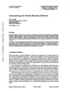
A typical vibro-acoustic duct is depicted on Fig.1. The geometry is axisymmetric and sketched on the (r,z) cutting plane. Ωa is the acoustic domain, Ωs the structural domain. Γc denotes the fluid/solid coupling interface. Boundary notations correspond to different types of boundary conditions, as defined later.
From now on and throughout this paper, a stationary, incompressible and homentropic base flow is assumed for simplicity. This implies that p0 remains spatially constant. Besides, a mixed pressure-displacement form is preferred to a purely displacement one, as justified later. In the harmonic case, equation (2.7) thus becomes: d 02 w L + ∇p L = 0 ρ0 2 dt p L = − ρ c 2∇ ⋅ w L 0 0
with:
d0 = −iω + v 0 ⋅∇ dt
(2.9)
When considering swirling flows, the constant p0 assumption cannot hold from the mean flow point of view because the azimuthal component of the flow velocity is
10
F. Treyssède, Acustica
directly related to the pressure gradient (see for instance Ref. 33). From the acoustical point of view, this assumption is less restrictive and means that terms in p0 gradient might have a negligible effect upon the acoustic propagation. The purpose of this paper is to get a simple validation of the FEM method to the detriment of fully realistic examples. However, as stated in Ref. 19 and 24, terms in p0 gradient should not
hal-01064471, version 1 - 16 Sep 2014
represent any numerical difficulties for the FEM method proposed in this paper.
A linear elastic and isotropic structure is assumed, with no initial stress and strain. The differential equation governing structure vibrations is thus given by:
ρs
∂ 2u − ∇ ⋅σ = 0 ∂t 2
(2.10)
ρs is the material density, u the structural displacement, σ the stress tensor. No external force density has been considered.
The coupling conditions that must be imposed at the fluid/solid interface are based upon the continuity of normal stress and normal displacement. According to Godin18, the continuity of the normal Lagrangian displacement is equivalent to the well-known Myers’ condition20, which holds when an Eulerian description is chosen. The coupling conditions are then: L u ⋅ n 0 = w ⋅ n 0 L σ ⋅ n 0 = − p n 0
on Γ c
(2.11)
n0 is the structure inward normal (outward from the fluid point of view), taken in the non-perturbed configuration.
11
F. Treyssède, Acustica
It is important to note that, given the fact that there is no initial stress and strain, no superscript are needed on the structural stress tensor and displacement because Eulerian and Lagrangian perturbations are equivalent in this specific case − see Eq. (2.3). It is the same for the fluid pressure fluctuation (we have assumed that p0 is constant). Thus, there is no ambiguity for the continuity of normal stresses, which is reduced to the well-known
hal-01064471, version 1 - 16 Sep 2014
normal stress continuity for vibro-acoustic problems.
For the acoustic part, we also need the two following boundary conditions: a fixed Lagrangian displacement condition and an absorbing wall condition. They are given by: w L = w on Γ w
w L ⋅ n0 = −
1 L p iω Z
(2.12) on Γi
(2.13)
Here again, the impedance condition is based on the normal displacement continuity. For a perfectly rigid wall, i.e. Z→∞, Eq. (2.13) reduces to w L ⋅ n 0 = 0 . For practical calculations, a third boundary condition may be needed at the outlet of the duct to simulate a modal non-reflecting condition, which is of the form: d0 w L ρ v ⋅ n = Znr ⋅ w L 0 ( 0 0) dt w L ⋅ n 0 = − 1 p L iω Z nr
on Γ nr
(2.14)
This condition has been successfully used in Ref. 19 and 24. Znr and Znr are respectively the standard modal non-reflecting impedance and the matrix impedance.
12
F. Treyssède, Acustica
The latter is needed to determine a unique solution when flow is present (a vector condition is necessary). Both impedances are explicitly given in section V.
For the structure, boundary conditions are of two types, a fixed displacement or a
hal-01064471, version 1 - 16 Sep 2014
fixed boundary force:
III.
u = u on Γ u
(2.15)
σ ⋅ n 0 = − f on Γ f
(2.16)
NUMERICAL METHOD
The variational formulation (already derived in Ref. 25) used for solving a general vibro-acoustic problem is first recalled. A mixed pressure-displacement based formulation is chosen for acoustics in order to avoid spurious solutions. The FEM discretisation of acoustic and structural variables is briefly given.
A. Variational formulation
For the acoustic part of the problem, the most natural variational formulation associated with Galbrun’ s equation is a purely displacement based formulation obtained from Eq. (2.7). However, this kind of formulation is known to give corrupted results when standard finite elements are used for discretisation, even in the no-flow case23,34.
13
F. Treyssède, Acustica
This locking phenomenon is analogous to what happens in fluid mechanics or structural mechanics when an incompressible medium is considered (see for instance Ref. 35). To avoid this problem, a mixed pressure-displacement based formulation has been proposed. More details are given in Ref. 24.
Equations (2.9) are respectively multiplied by two trial fields, w* and p*, and
hal-01064471, version 1 - 16 Sep 2014
integrated over the acoustic domain Ωa. After integrating by parts, we get:
1 * L p p dΩ+ ∫ ∇p* ⋅ wLdΩ+ ∫ w* ⋅∇pLdΩ−ω2 ∫ ρ0w* ⋅ wLdΩ 2 ρc Ωa 0 0 Ωa Ωa Ωa
−∫
−iω ∫ ρ0w* ⋅(v0 ⋅∇wL )dΩ+iω ∫ ρ0 (v0 ⋅∇w* )⋅ wLdΩ Ωa
Ωa
− ∫ ρ0 (v0 ⋅∇w* )⋅(v0 ⋅∇wL )dΩ
(3.1)
Ωa
dwL * L * * + ∫ w* ⋅ ρ0 (v0 ⋅n0 ) dS − ∫ p (w ⋅n0 )dS = 0 ∀{w , p } dt ∂Ωa ∂Ωa where ∂Ωa is the surface enclosing the acoustic domain Ωa.
In the no-flow case (first line of the above formulation), the domain operators of (3.1) are almost identical to those used by Wang and Bathe36 in their mixed formulation. The only slight difference is that one has chosen to integrate by parts the divergence term of the second equation of system (2.9) (instead of the last term of the first equation) in order to let the normal displacement appear explicitly at the boundary.
As noted in Ref. 25, normal displacement continuity is then easily imposed by replacing the fluid normal displacement with the structure normal displacement when
14
F. Treyssède, Acustica
fluid-structure interactions are considered. This specificity avoids the use of a Lagrangian multiplier to force normal displacement continuity, as done in Ref. 30 and 37.
The variational formulation associated to the structure equation (2.10) does not present any problem. It is classically obtained after multiplication by a trial field u* and
hal-01064471, version 1 - 16 Sep 2014
integrating by parts:
∫ε
Ωs
*
: σ dΩ−ω2 ∫ ρsu* ⋅ udΩ+ Ωs
∫ u ⋅(σ ⋅n )dS *
0
= 0
∀u*
(3.2)
∂Ωs
where ∂Ωs is the surface enclosing the structural domain Ωs, ε the symmetric strain tensor (n0 is still the inward normal from the structure point of view).
Now, formulations (3.1) and (3.2) are combined. Vibro-acoustic coupling conditions (2.11) are applied by replacing the acoustic normal displacement in the boundary integral over Γc of (3.1), and the structural normal stress tensor in the boundary integral over Γc of (3.2). Boundary conditions (2.12), (2.14) and (2.15) are also applied. This yields the following general vibro-acoustic variational formulation, which consists in
{
solving {w L , p L , u} verifying w L
Γw
}
= w and u Γ = u and: u
15
F. Treyssède, Acustica
1 * L p p dΩ+ ∫ ∇p* ⋅ wLdΩ+ ∫ w* ⋅∇pLdΩ−ω2 ∫ ρ0w* ⋅ wLdΩ 2 ρc Ωa 0 0 Ωa Ωa Ωa
−∫
−iω ∫ ρ0w* ⋅(v0 ⋅∇wL ) dΩ+ iω ∫ ρ0 ( v0 ⋅∇w* )⋅ wLdΩ− ∫ ρ0 (v0 ⋅∇w* )⋅(v0 ⋅∇wL ) dΩ Ωa
Ωa
− ∫ p* (wL ⋅n0 ) dS + Γw
Ωa
1 1 * L 1 1 * L p p dS + ∫ w* ⋅(Znr ⋅ wL ) dS + ∫ p p dS ∫ iω Γi Z iω Γnr Znr Γnr
(3.3)
−ω2 ∫ ρsu* ⋅udΩ+ ∫ ε* :σdΩ+ ∫ u* ⋅ fdS Ωs
Ωs
Γf
−∫ p* (u⋅n0 ) dS − ∫ (u* ⋅n0 ) pLdS = 0 Γc
{
∀w*, p*,u* w*
Γc
Γw
}
= 0 and u* = 0 Γu
hal-01064471, version 1 - 16 Sep 2014
The three first lines represent the acoustic problem when no coupling is assumed, the fourth line is the structural problem and the last line gives coupling conditions between both media. Note that impermeable walls have been assumed so that v 0 ⋅ n 0 = 0 on Γc∪Γi.
It is interesting to note that both the impedance condition (2.12) and the normal displacement continuity (2.11) are based upon the equality of the explicit variable w L ⋅ n 0 = 0 with the wall normal displacement. These conditions are then much simpler
to implement than in the LEE case, that would have required the use of Myer’ s condition (in particular, Myer’ s condition implies normal derivatives, which are difficult to compute via a FEM method).
B. Finite element discretization
16
F. Treyssède, Acustica
In this paper, the geometry is assumed to be axisymmetric. Without loss of generality, fluctuating variables can be written in the following form:
(w , p , u)(r,θ , z, t ) = (w , p , u)(r, z )e ( L
L
L
i mθ −ωt )
L
(3.4)
Trial functions are given by:
(w , p , u )(r,θ , z, t ) = (w , p , u )(r, z)e ( *
*
*
*
*
*
−i mθ −ωt )
(3.5)
In order to avoid locking and spurious solutions, a mixed pressure-displacement
hal-01064471, version 1 - 16 Sep 2014
formulation is not sufficient: interpolations for displacement and pressure variables must be adequately chosen. Though not necessary, a criterion that ensures convergence and stability of the finite element is given by the inf-sup condition (see for instance Ref. 35). This kind of finite element has already been successfully applied to the variational formulation (3.3) in the no-flow case36 and when testing the effect of shear flows24,25. The element used in this paper, sometimes referred to as the “P1+-P1”, “4/3c” or “MINI” element in the literature, is a three-node triangle with an internal degree of freedom for each component of the displacement. On the reference element, displacement and pressure variables are thus interpolated as follows:
wL (u, v) = (1− u − v) w1 + uw2 + vw3 + (1− u − v)uva L p (u, v) = (1− u − v) p1 + up2 + vp3
(3.6)
where the subscripts i (i=1,2,3) denotes the node number. The standard linear interpolation for the displacement is enriched with a bubble function that maintains C0 continuity (a is a generalised variable corresponding to an internal degree of freedom, which can be condensed out before the elements are assembled). As a side remark, it has
17
F. Treyssède, Acustica
to be noted that the overall method presented in this paper is easily applicable to the 3D case because elements satisfying the inf-sup condition exists in three dimensions too35.
The structure is assumed to be a thin shell of constant thickness, described with Reissner/Mindlin’ s theory. To avoid transverse shear locking, the variational formulation associated to the structure is also mixed, written with displacements and rotations as
hal-01064471, version 1 - 16 Sep 2014
explicit variables (a linear interpolation is chosen for each). A complete description of such an element is given for an axisymmetric shell geometry in Ref. 38, p.196.
After assembling and applying boundary conditions, the global discretised variational formulation yields an algebraic system of the form:
K a CT
C uˆ a fa = K s uˆ s fs
(3.7)
where uˆa and uˆs respectively contain all the acoustic nodal unknowns (i.e. displacement and pressure) and all the structural unknowns (displacement and rotation). C is the fluid/structure coupling matrix. fa and fs denote the acoustic and vibration sources. Some more details are provided in Ref. 25. The overall left-hand matrix in (3.7) is ωdependent, unsymmetrical, complex and banded. A sparse storage is chosen. For a fixed
ω, the unknown nodal vector is finally obtained by using a LU decomposition.
18
F. Treyssède, Acustica
IV.
SEMI-ANALYTICAL MODEL
This section presents the semi-analytical model used for the validation of the FEM model. This model constitutes a sort of Pridmore-Brown equation generalized to a swirling flow. It corresponds to the propagation of a single mode in a straight duct. Extending Pagneux and Aurégan’ s work to non-axisymmetric modes, the effect of a
hal-01064471, version 1 - 16 Sep 2014
vibrating wall is also included in order to study vibro-acoustic coupling.
A. Acoustic
For the acoustic fluid, we first suppose that p0 is constant and that the flow speed components only depend upon r (with no radial velocity):
v 0 = v0 (r )e z + rω 0 (r )eθ
, ρ 0 = ρ 0 (r )
(4.1)
ω0(r) is the rotation speed (in rad/s) of the mean flow at r. Fluctuating fields are written with the following dependence:
(w , p )(r,θ , z, t ) = (w , p )(r )e ( L
L
L
L
i kz z +mθ −ωt )
(4.2)
where kz denotes the axial wave number. The material derivative is now given by
d 0 dt = −i (ω − v0 k z − mω 0 ) . The system (2.9) becomes:
19
F. Treyssède, Acustica
∂p L 2 L − Ω + =0 ρ w r 0 ∂ r − ρ Ω 2 wL + i m p L = 0 θ 0 r L 2 L − ρ 0 Ω wz + ik z p = 0 ∂ (rwrL ) m L 2 1 L L ρ = − + + p c i w ik w 0 0 θ z z r r r ∂
(4.3)
with Ω (r ) = ω − v0 (r ) k z − mω 0 (r ) . The first three equations allow to explicitly express
hal-01064471, version 1 - 16 Sep 2014
the Lagrangian displacement in terms of the pressure. Then replacing displacement in the last equation of (4.3) yields the following scalar second order differential equation:
∂2 pL 1 Ω′ ρ 0′ ∂p L Ω 2 m 2 + − 2 − + 2 − 2 − k z2 p L = 0 2 ∂r Ω ρ 0 ∂r c0 r r
(4.4)
The primes denotes r-derivatives. In a way, Eq. (4.4) represents a Pridmore-Brown equation generalised to swirling flows.
Using the first equation of (4.3), boundary condition (2.12) at r=R1 and r=R2 becomes:
∂p L ∂r
r = R1,2
ρ 0Ω2 L = Bi p ω Z1,2
(4.5)
Signs − and + are respectively associated with indices 1 and 2. Note that Eq. (4.5) reduces to the no-flow case boundary condition ∂p L ∂r = Bi ρ0ω p L Z1,2 only if the mean flow velocity is zero at walls (non-slip condition).
20
F. Treyssède, Acustica
Equations (4.4) and (4.5) constitutes an eigenvalue problem, whose eigenvalues and eigenfunctions are respectively kz and pL(r). Its solution requires a numerical method and leads to the wave modes. In this paper, it is assumed that ρ 0′ = 0 (incompressible case) for simplicity as stated earlier. Besides, it must be noted that the constant p0 assumption made earlier is important for obtaining the relatively simple Eq. (4.4). Indeed, if p0 is rdependent, a scalar differential equation written only in terms of a single variable
hal-01064471, version 1 - 16 Sep 2014
(namely p or wrL ) may still be found9,22 but calculations are tedious and this equation is far more complex than (4.4).
B. Vibro-acoustic coupling
In case of coupled vibrating walls, the boundary condition (4.5) is modified. This subsection is an extension to rotating modes ( m ≠ 0 ) of Pagneux and Aurégan’ s paper29. The assumption of a thin shell based on Kirchhoff theory is made. Vibration equations of a fluid-loaded wall located at r=Ri (i=1,2) are then governed by Donnell’ s theory39: ν ∂ur 1 + ν ∂ 2uθ ∂ 2 1 − ν ∂ 2 1 ∂2 + + + − u =0 2 2 2 2 2 z ∂ ∂ ∂ ∂ ∂ ∂ θ θ 2 2 R z R z z R c t i i i L 2 1 ∂2 1 ∂2 1 + ν ∂ 2u z 1 ∂ur 1 − ν ∂ + + − + =0 u 2 θ 2 2 Ri ∂θ∂z Ri2 ∂θ 2 cL2 ∂t 2 Ri ∂θ 2 ∂z 2 1 + β 2∇ 4 + 1 ∂ ur + 1 ∂uθ + ν ∂u z = B 1 p L r = Ri Ri2 ρ s hcL2 cL2 ∂t 2 Ri2 ∂θ Ri ∂z
i = 1, 2
(4.6)
Signs − and + are respectively associated with indices 1 and 2. cL, β and ∇4 are defined as:
21
F. Treyssède, Acustica
cL2 =
E h2 2 , β = 12 Ri2 ρ s (1 −ν 2 )
, ∇ 4 = Ri2
1 ∂4 ∂4 ∂4 2 + + ∂z 4 ∂θ 2 ∂z 2 Ri2 ∂θ 4
(4.7)
E, ρs, ν, h and cL are respectively the Young’ s modulus, density, Poisson’ s ratio, thickness and longitudinal wave speed of the shell being considered.
With the same dependence as in (4.2), structural displacements are re-written: u (r,θ , z, t ) = u (r )e ( z
hal-01064471, version 1 - 16 Sep 2014
i k z +mθ −ωt )
(4.8)
Equation (4.6) now becomes: 2 i ν k u − 1 + ν mk u + − k 2 − 1 −ν m 2 + ω u = 0 z z z θ Ri z r 2 Ri 2 Ri2 cL2 m 1 −ν 2 m 2 ω 2 1 +ν k z − 2 + 2 uθ − mk z u z = 0 i 2 ur + − 2 2 Ri Ri cL Ri 2 2 2 1 + β 2 R 2 k 2 + m − ω u + i m u + i ν k u = B 1 p L r θ i z z z R 2 ρ s hcL2 Ri2 cL2 Ri2 Ri i
i = 1, 2 (4.9)
r = Ri
The above three equations allow to write ur in terms of pL(r=Ri) only. After calculations, it can be shown that: m ν (1 + ν ) 2 k z + 1 ur uθ = −i 2 Ri α 2 2α1 u = −i 1 1 + ν m 2 k ν (1 + ν ) k 2 + 1 + ν k u i = 1, 2 z z z r z Riα1 2 Ri2α 2 2α1 (4.10) 2 2 2 2 ν k z (1 + ν ) m2 k 2 + 1 + m ν (1 + ν ) k 2 + 1 z z Ri2α1 4 Ri2α1α 2 Ri4α 2 α1 2 2 ω 2 m 1 1 2 2 2 + 2 + β Ri k z + 2 − 2 ur = B pL 2 r = Ri ρ s hcL Ri Ri cL
22
F. Treyssède, Acustica
where:
ω2 1 −ν ω 2 (1 + ν ) 2 2 1 −ν 2 m2 α1 = 2 − k z2 − 2 m 2 , α 2 = 2 − m kz − kz − 2 2 Ri 4 Ri2α1 2 cL cL Ri 2
(4.11)
Then, using the first equation of (4.3) and the normal continuity displacement, i.e. wrL = ur at r=Ri, the last equation of (4.10) finally gives:
hal-01064471, version 1 - 16 Sep 2014
2 2 2 m 2 ν (1 + ν ) 2 ν k z (1 + ν ) 2 2 1 m k k z + 1 + + 4 2 2 z Ri α 2 α1 4 R R α α α 1 1 2 i i 2 1 m 2 ω 2 ∂p L 2 2 2 + 2 + β Ri k z + 2 − 2 Ri Ri cL ∂r
(4.12) =B r = Ri
ρ 0Ω L p r = Ri ρ s hcL2 2
Equation (4.12) constitutes the boundary condition that must be used to solve the differential equation (4.4) when coupling effect of the vibrating wall r=Ri has to be included in the analysis.
C. Solution method
In order to solve Eq. (4.4) combined with (4.5) or (4.12), the solution of the specific case of a uniform axial flow and rigid-body rotation is first obtained. Then, the solution for kz is used as an initial value to solve the more general equation (4.4) with an iterative Runge-Kutta method.
23
F. Treyssède, Acustica
The specific solution uniform/rigid-body implies that r-derivatives of Ω become zero. Solutions of Eq. (4.4) in the constant ρ0 case are thus a combination of Bessel’ s functions:
(
)
(
L pmn (r ) = AJ m krmn r + BYm krmn r
)
(4.13)
where the radial wave number is given by the dispersion equation:
kr2mn = Ω 2 c02 − k z2mn
(4.14)
hal-01064471, version 1 - 16 Sep 2014
With γi being a factor that depends on the type of conditions used, (4.5) or (4.12), boundary conditions are of the form: ∂p L ∂r
= γ i pL
(4.15)
r = Ri
Then, application of (4.13) into (4.15) yields the following characteristic equation:
{k J ′ (k R ) − γ J (k R )}{k Y ′ (k R ) − γ Y (k R )} − {k J ′ (k R ) − γ J (k R )}{k Y ′ (k R ) − γ Y (k R )} = 0 rmn
m
rmn
rmn
m
1
rmn
1 m
2
2
rmn
m
1
rmn
rmn m
2
rmn m
2
rmn
rmn
2 m
1
1 m
2
rmn
rmn
(4.16)
1
The nth solution gives the axial wave number kz of the mode (m,n−1). Besides, it can be shown from (4.14) that:
k
± zmn
=
− M 0 (k − mk0 ) ±
(k − mk0 )
2
1 − M 02
− (1 − M 02 ) kr2mn
(4.17)
where k=ω/c0, M0=v0/c0 and k0=ω0/c0. This relation is the same that is in Kerrebrock’ s analysis5. Cut-off frequencies of the (m,n) mode corresponds to the value of k for which the term inside the square root vanishes when perfectly rigid walls are considered. After some calculations, we have:
24
F. Treyssède, Acustica
f cmn = 1 − M 02 f 0mn +
mω 0 2π
(4.18)
f 0mn = c0 krmn 2π is the no-flow cut-off frequency. This simple relation shows that
cut-off frequencies are modulated by a
1 − M 02 factor (for any direction of the axial
flow) and incremented by mω 0 2π (cut-off frequencies of counter-rotating modes are decreased, and vice-versa for co-rotating modes). This basic result will be experienced in
hal-01064471, version 1 - 16 Sep 2014
the next section.
If the mode is cut-off or duct walls are lined, kz becomes complex, which means that the mode is attenuated. This attenuation is given in dB/m by:
α = 8.686 Im (k z )
V.
(4.19)
RESULTS
Figure 1 shows the types of boundary conditions used for FEM calculations. The methodology is as follows. Lagrangian displacements obtained from the semi-analytical model are imposed at the duct inlet of the FEM model (in the remaining, the term “ inlet” is used for the bottom z=0 cross-section). The modal non-reflective boundary condition (2.14) is preferred at the outlet, which is less constraining because phase and amplitude are left free. FEM solutions inside the duct are then computed and compared to the semianalytical ones.
25
F. Treyssède, Acustica
Impedances defined by (2.14) can be given explicitly for a single mode, for which an ei (k z − mθ −ωt ) dependence is assumed (as described in section IV). Material derivatives are z
thus simply given by d/dt=−i(ω−v0kz−mω0), which yields the following explicit expressions:
hal-01064471, version 1 - 16 Sep 2014
Znr = −i ρ0v0 (ω − v0 kz − mω0 )I , Znr = ρ0
(ω − v0kz − mω0 )
2
ω kz
(5.1)
kz is the modal axial wave-number, which is part of the semi-analytical solution. I denotes the identity matrix.
When vibro-acoustics problems are considered, semi-analytical displacements and rotations are also enforced at the shell extremities of the FEM model. Semi-analytical displacements are obtained from the semi-analytical pressure with (4.10). With notations of section IV, semi-analytical rotations in the (r,z) and (x,y) planes, denoted by β and βθ, are calculated as follows:
β = ikz ur , βθ = (imur − uθ ) Ri
(5.2)
It is important to note that the above relations suppose that there is no transverse shear because the Kirchhoff’ s theory has been used in Section IV. In particular, a rather small shell thickness has to be chosen in order for both models to converge (as stated earlier, the shell FEM model takes into account any possible transverse shear).
26
F. Treyssède, Acustica
In the following, iso-pressure contours are given in Pa in order not to minimize errors. Axial mean flow velocities are defined in Mach number (M0). Mean flow rotations are given with a non-dimensional parameter defined as: Ω0 = ω0 ( R2 − R1 ) c0
(5.3)
where R1 and R2 are the inner and outer duct radius. Propagation and axial flow directions are also sketched in order to explicitly show if wave propagation is upstream
hal-01064471, version 1 - 16 Sep 2014
or downstream. Typical values of ρ0=1.2kg.m-3 and c0=340m.s-1 are used.
Test cases sweep a non-dimensional frequency range up to about kR=15 and the duct geometry is generally meshed with a λ/10 finite element length. Meshes may be adequately refined at walls in order to better describe the effects of the mean flow boundary layer thickness as well as shell vibrations, as done in Ref. 25. Figure 2 gives an example of a λ/10 meshing, without and with refinement, used for the results of Fig.6 (f=650Hz).
A. Validation for pure acoustic propagation
The first test case is a (±3,1) mode propagating at f=400Hz in a cylindrical duct of radius R2=1.0m (R1=0), with perfectly rigid walls, with a uniform axial mean flow and a rigid-body rotation represented by:
v0z (r ) = M 0c0 , v0θ (r ) = Ω0c0 r ( R2 − R1 )
27
(5.4)
F. Treyssède, Acustica
where M0 and Ω0 are both constant. Here, we choose M0=+0.3 and Ω0=+0.3.
A comparison between semi-analytical and FEM solutions is shown on Fig.3 for m=−3 (counter-rotating mode) and m=+3 (co-rotating). A good convergence between both models is achieved, though small discrepancies can be observed on Fig.3b near the modal pressure node (at r=0.8m). As shown on Fig.4, those numerical discrepancies
hal-01064471, version 1 - 16 Sep 2014
almost disappear when the mesh is refined (λ/10 and λ/20 meshes have been used for Fig.3b and 4 respectively). However, analyses of convergence of the FEM implementation will not be pursued in this paper and are left for further studies40,41.
It can be observed that the counter-rotating mode fully propagates along the duct whereas the co-rotating mode is quickly damped near the duct inlet, indicating that this mode is cut-off. This is confirmed by Eq. (4.18), which yields cut-off frequencies fc=365Hz for m=−3 and 462Hz for m=+3 (the no-swirl mode would have been cut-off also because fc=414Hz). This example simply shows the effects of swirl upon cut-off frequencies, which are well taken into-account by the FEM model.
A second test case concerns a (±10,0) mode propagating at f=650Hz in an annular duct of radius R1=0.2m and R2=1.0m. The mean flow is assumed to have a sheared axial velocity with M 0 = −0.5 and a 10% boundary layer thickness (δ=0.08m, the profile is assumed to be parabolic – see Fig.5). The mean flow also has a rigid-body rotation with a free vortex. The azimuthal velocity is explicitly given by:
28
F. Treyssède, Acustica
v0θ (r ) = Πr + Γ r
(5.5)
Π and Γ are two constants chosen so that Γ Π = 0.32 and Ω0 = +0.1 . M 0 and Ω0 are the cross-section averages of M 0 (r) and Ω0 (r), defined by: f =
2π R2
1 2 π (R2 − R12 ) ∫0
∫ f (r ) rdrdθ
(5.6)
R1
hal-01064471, version 1 - 16 Sep 2014
Figure 5 illustrates some velocity profiles for M 0 = 0.4 and Ω0 = 0.2 .
The outer wall is lined, with Z=2040−2040i. As seen on Fig.6, this example exhibits strong differences in attenuation between cases m=−10, m=10 (no swirl), and m=+10. It must be emphasised that attenuation is only due to the lining effect because the frequency f=650Hz has been carefully chosen so that the (±10,0) modes are always cuton (even for m=+10, fc=619Hz). This is illustrated by the non-zero intensity, also shown on Fig.6 and post-processed via Eq. (2.8). Note that the intensity vector is not perfectly tangential to the wall, indicating that some energy is absorbed by the lining. Results obtained from both semi-analytical and FEM models are still satisfyingly in agreement, though a slight difference may be observed in the counter-rotating case. Moreover, the conclusion of this example agrees with Cooper and Peake’ s results10 obtained in lined ducts: a co-rotating mode may be much more damped than in the no-swirl case, a counter-rotating mode is generally less attenuated. Attenuation may be quantified precisely by the semi-analytical solution – see Eq. (4.19). Attenuation factors found for m=−10, m=10 (no swirl), and m=+10 are respectively 2.8dB/m, 5.3dB/m and 11.6dB/m.
29
F. Treyssède, Acustica
Consequently, neglecting swirl for acoustic propagation may lead to significant errors, especially for counter-rotating modes because their attenuation will be overestimated. It must be noted that the uniform case (i.e. uniform axial velocity and rotation) would have given quite different values of attenuations (respectively: 9.1, 11.2 and 20.5dB/m – not shown here). The FEM model gives therefore a good accuracy of convection and
hal-01064471, version 1 - 16 Sep 2014
refraction effects due to radial variation of flow velocities.
B. Validation for vibro-acoustic coupling
In this section, the outer wall is now elastic. Material is aluminium. Shell characteristics are as follows: E=7.0×10¹⁰N/m2, ρs=2700kg/m3, ν=0.3, h=0.01m.
The first vibro-acoustic example is given by Fig.7-9. The test geometry and flow are the same that in the first example of the preceding subheading: a cylindrical rigid wall duct with uniform flow/rigid-body rotation is considered (M0=+0.3 and Ω0=+0.3). One is interested in the (±5,0) mode propagating at f=500Hz (this mode is always cut-on at this frequency – for m=+5, fc=412Hz). Figure 7 gives a comparison for m=−5, m=5 (no swirl), and m=+5. Note that the pressure real part have been preferred instead of the modulus because the latter is almost identical for the three cases, which would not have been very useful to show. In addition to the fact that semi-analytical and FEM solutions perfectly coincide, it may be observed that mode radial profiles do not change with the
30
F. Treyssède, Acustica
sign of mΩ0 (i.e. between co- and counter-rotating cases). However, as expected, the axial wave number is strongly reduced for m>0, explaining the axial wavelength increasing from left to right on Fig.7. As shown on Fig.8, this decrease of kz is accompanied by a decrease of the axial intensity from 10-3W/m2 for m=−5 to about 0.6×10⁻³W/m2 for m=+5 (on the other hand, there is an increase of the azimuthal
hal-01064471, version 1 - 16 Sep 2014
component).
Figure 9 shows the real part of the shell radial displacement. An interesting swirl effect can be viewed: when the mode is counter-rotating, the radial displacement is far greater than for the no-swirl mode. In the co-rotating case, the radial displacement is lower, but the difference is rather slight. The shell radial displacement is multiplied by about a factor 10 between m=+5 and m=−5. Note that semi-analytical and FEM displacements perfectly coincide (for a simpler visibility of Fig.9, one has chosen the same line styles for both models).
Nevertheless, the above result must not be generalised. The opposite can also be observed. Figure 10 exhibits the shell radial displacement for an upstream propagation M0=−0.3 (pressure has not been shown for this example). The co-rotating mode radial displacement is, this time, amplified compared to the counter-rotating one by a factor 4. The above results simply shows that mean swirl effects may be strong upon vibroacosutic behaviours and need to be included in engineering analyses.
31
F. Treyssède, Acustica
The last example illustrates the capabilities of the FEM model to adequately include the effects of radial variations of the mean flow for higher frequencies. For that purpose, Fig.11 gives a comparison between a non-uniform and a uniform flow. The duct is annular, with R1=0.2m and R2=1.0m. The non-uniform flow is of the same type that the one used for the second test case of the last subheading, but with M 0 = −0.4 and
Ω0 = +0.2 . The uniform flow corresponds to the same averages, as defined by (5.6)
hal-01064471, version 1 - 16 Sep 2014
(what must be understood by “ uniform” flow is that both axial velocity and rotation are uniform). Figure 5 exhibits uniform and non uniform flow profiles for the axial and azimuthal velocities. The case of a (+2,3) mode propagating at f=1000Hz with an inner lined wall is considered. The impedance wall is Z=408−408i.
The attenuation due to the lining is slightly more pronounced in the non-uniform case. Attenuations obtained from the semi-analytical solutions yield the values of 1.0dB/m for the non-uniform flow and 2.4dB/m for the uniform case. Though radial variations of both M0(r) and Ω0(r) may generally play a significant role, a further analysis shows that, for the case being considered, the difference of attenuation is mainly due to the presence of axial flow shear. For an upstream propagation, the aerodynamic boundary layer tends to refract waves away from the walls, decreasing the efficiency of the lining. This gives a non-negligible difference of about 3dB at the duct outlet (L=2m). Given the rather good agreement between both models, the FEM method proposed in this paper is able to support the convection/refraction effects of complex flows. Figure 12 also gives the shell radial displacements in order to observe the decrease of the
32
F. Treyssède, Acustica
structural vibration along the duct. Attenuation difference existing between both kinds of flow is slight but well represented by the FEM model.
At last, it should be noted that Fig.11a-b and 12 exhibit some small differences between MS and FEM solutions (however, note that if plots were given in dB, errors between both models would be almost negligible). As explained at the beginning of
hal-01064471, version 1 - 16 Sep 2014
Sec.V, the FEM models have been meshed with a λ/10 length, which constitutes an estimated finite element length for acceptable convergence. As done for Fig.3b and 4, convergence may be further improved by a mesh refinement (not shown here for conciseness of the paper).
VI.
CONCLUSION
In this paper, a FEM model based on Galbrun’ s equation has been proposed to solve acoustic and vibro-acoustic problems in the presence of swirling (and sheared) flows. From a theoretical and numerical point of view, Galbrun’ s equation may be attractive compared to the LEE: boundary conditions are easy to obtain and to implement with a FEM method, and an exact intensity expression is available. Moreover, the proposed variational formulation is well suited to enforce the fluid/structure coupling conditions.
Through comparisons with semi-analytical solutions based on a generalised Pridmore-Brown equation, the swirl effects upon acoustic and vibro-acoustic behaviours
33
F. Treyssède, Acustica
have been outlined and the FEM method was tested. The agreement between both models tends to prove that the proposed method is efficient to study such applications.
Results also show the importance of taking into account swirling flows, and therefore, the limitations inherent to a full-potential formulation, which assumes that both acoustic and aerodynamic velocities are irrotational. This justifies the use of more
hal-01064471, version 1 - 16 Sep 2014
general equations, such as the LEE or Galbrun’ s equation. In particular, co-rotating (resp. counter-rotating) modes are likely to be more (resp. less) damped along a lined duct than in the no-swirl case. The presence of swirl may also strongly affect the structural vibrations by sometimes increasing, sometimes decreasing, their radial displacement amplitudes.
1
S. J. Horowitz, R. K. Sigman, and B. T. Zinn, “ An iterative finite element-integral technique for predicting sound radiation from turbofan inlets in steady flight,” American Institute of Aeronautics and Astronautics Journal 24, 1256-1262 (1986).
2
P. Zhang, T. Wu, and L. Lee,. “ A coupled FEM/BEM formulation for acoustic radiation in a subsonic non-uniform flow,” Journal of Sound and Vibration 192, 333347 (1996).
3
W. Eversman, and D. Okunbor, “ Aft fan duct acoustic radiation,” Journal of Sound and Vibration 213, 235-257 (1998).
34
F. Treyssède, Acustica
4
S. W. Rienstra, and W. Eversman, “ A numerical comparison between the multiplescales and finite-element solution for sound propagation in lined flow ducts,” Journal of Fluid Mechanics 437, 367-384 (2001).
5
J. L. Kerrebrock, “ Small disturbances in turbomachine annuli with swirl,” American Institute of Aeronautics and Astronautics Journal 15, 794-803 (1977).
6
M. Roger, and H. Arbey, “ Champ de pression dans un conduit annulaire en présence
hal-01064471, version 1 - 16 Sep 2014
d’ un écoulement tournant de rotation solide” (“ Pressure field in a fluid in solid body rotation” ), Revue d’ Acoustique 16, 240-242 (1983). 7
M. Roger, and H. Arbey, “ Relation de dispersion des ondes de pression dans un écoulement tournant” (“ Dispersion relation of pressure waves in a swirling flow” ), Acustica 59, 95-101 (1985).
8
V. Golubev, and H. M. Atassi, “ Acoustic-vorticity waves in swirling flows,” Journal of Sound and Vibration 209, 203-222 (1998).
9
C. K. W. Tam, and L. Auriault, “ The wave modes in ducted swirling flows” , Journal of Fluid Mechanics 371, 1-20 (1998).
10
J. Cooper, and N. Peake, “ Propagation of unsteady disturbances in a slowly varying duct with mean swirling flow,” Journal of Fluid Mechanics 445, 207-234 (2001).
11
L. Abrahamson, “ A finite element algorithm for sound propagation in axisymmetric ducts containing compressible mean flow,” AIAA 4th Aeroacoustics Conference, Atlanta (1977).
35
F. Treyssède, Acustica
12
R. J. Astley, and W. Eversman, “ Acoustic transmission in non-uniform ducts with mean flow, part II: the finite element method,” Journal of Sound and Vibration 74, 103-121 (1981).
13
R. J. Astley, and W. Eversman, “ A finite element formulation of the eigenvalue problem in lined ducts with flow,” Journal of Sound and. Vibration 65, 61-74 (1979).
14
L. Greverie, and C. Bailly, “ Construction d’ un opérateur de propagation à partir des
hal-01064471, version 1 - 16 Sep 2014
équations d’ Euler linéarisées” (“ Formulation of an acoustic wave operator based on linearized Euler equations” ), Comptes-rendus de l’ Académie des Sciences Série IIb 326, 741-746 (1998). 15
Longatte, and P. Lafon, “ Computation of acoustic propagation in two-dimensional sheared ducted flow,” American Institute of Aeronautics and Astronautics Journal 38, 389-394 (2000).
16
Bailly, and D. Juve, “ Numerical solution of acoustic propagation problems using linearized Euler equations,” American Institute of Aeronautics and Astronautics Journal 38, 22-29 (2000).
17
H. Galbrun, Propagation d’Une Onde Sonore Dans l’Atmosphère et Théorie des Zones de Silence (Propagation of an acoustic wave in the atmosphere and theory of zones of silence) (Gauthier-Villars, Paris, 1931).
18
O. A. Godin, “ Reciprocity and energy theorems for waves in a compressible inhomogeneous moving fluid,” Wave Motion 25, 143-167 (1997).
19
Peyret, and G. Elias, “ Finite-element method to study harmonic aeroacoustics problems,” Journal of the Acoustical Society of America 110, 661-668 (2001).
36
F. Treyssède, Acustica
20
M. K. Myers, “ On the acoustic boundary condition in the presence of flow,” Journal of Sound and Vibration 71, 429-434 (1980).
21
Poiree, “ Les équations de l’ acoustique linéaire et non linéaire dans un écoulement de fluide parfait” (“ Equations of linear and non linear acoustics in a perfect fluid flow” ), Acustica 57, 5-25 (1985).
22
B. Poirée, “ Petites perturbations d’ un écoulement tournant” (“ Small perturbations in a rotating flow” ), Acustica 59, 85-94 (1985).
hal-01064471, version 1 - 16 Sep 2014
23
S. Bonnet-Ben Dhia, G. Legendre, and E. Luneville, “ Analyse mathématique de l’ équation de Galbrun en écoulement uniforme” (“ Mathematical analysis of Galbrun’ s equation with uniform flow” ), Comptes-rendus de l’ Académie des Sciences Série IIb 329, 601-606 (2001).
24
F. Treyssède, G. Gabard, and M. Ben Tahar, “ A mixed finite element method for acoustic wave propagation in moving fluids based on an Eulerian-Lagrangian description,” Journal of the Acoustical Society of America 113, 705-716 (2003).
25
G. Gabard, F. Treyssède, and M. Ben Tahar, “ A numerical method for vibro-acoustic problems with sheared mean flows” , accepted in the Journal of Sound and Vibration.
26
D. C. Crighton, and J. E. Oswell, “ Fluid loading with mean flow. I. Response of an elastic plate to localized excitation,” Philosophical Transactions of the Royal Society A 335, 557-592 (1991).
27
F. Sgard, N. Atalla, and J. Nicolas, “ Coupled BEM-FEM approach for mean flow effects on vibro-acoustic behavior of planar structures,” American Institute of Aeronautics and Astronautics Journal 32, 2351-2358 (1994).
37
F. Treyssède, Acustica
28
N. Ouelaa, B. Laulagnet, and J.-L. Guyader, “ Etude vibro-acoustique d’ une coque cylindrique finie remplie de fluide en mouvement uniforme” (“ Vibro-acoustic analysis of a finite cylindrical shell carrying uniform mean flow” ), Acustica 2, 275289 (1994).
29
V. Pagneux, and Y. Aurégan, “ Acoustic modes in duct with parallel shear flow and vibrating walls,” Fourth AIAA/CEAS Aeroacoustics Conference Paper No. 98-2281 (1998).
hal-01064471, version 1 - 16 Sep 2014
30
M. Ben Tahar, and E. Goy, “ Resolution of a vibroacoustic problem in the presence of a nonuniform mean flow,” Fourth AIAA Joint Aeroacoustics Conference Paper No. 98-2215 (1998).
31
B. Poirée, “ Les équations de l’ acoustique linéaire et non-linéaire dans les fluides en mouvement” (“ Equations governing linear and non-linear acoustics in moving flows” ), Thèse d’ état, Université Pierre et Marie Curie, Paris 6, 1982.
32
Blokhintzev, “ The propagation of sound in an inhomogeneous and moving medium I,” Journal of the Acoustical Society of America 18, 322-328 (1946).
33
G. K. Batchelor, An Introduction To Fluid Dynamics (Cambridge Press University, 1967).
34
M. A. Hamdi, and Y. Ousset, “ A displacement method for the analysis of vibrations of coupled fluid-structure systems,” International Journal for Numerical Methods in Engineering 13, 139-150 (1978).
35
K. J. Bathe, Finite Element Procedures (Prentice Hall, Englewood Cliffs, 1996).
38
F. Treyssède, Acustica
36
X. Wang, and K. J. Bathe, “ Displacement/Pressure based mixed finite element formulations for acoustic fluid-structure interaction problems,” International Journal for Numerical Methods in Engineering 40, 2001-2017 (1997).
37
Bermudez, and L. Hervella-Nieto, “ Finite element computation of three-dimensional elastoacoustic vibrations,” Journal of Sound and Vibration 219, 279-306 (1999).
38
J.-L. Batoz and G. Dhatt, Modélisation des Structures par Eléments Finis – Coques (Structural design with finite element methods - shells) (Hermès, Paris, 1992).
hal-01064471, version 1 - 16 Sep 2014
39
C. Lesueur, Rayonnement Acoustique des Structures - Vibro-acoustique, Interactions Fluide/Structure
(Acoustics
radiation
from
structures
-
vibro-acoustics,
fluid/structure interactions) (Eyrolles, Paris, 1988). 40
G. Gabard, R.J. Astley, and M. Ben Tahar, “ Stability and accuracy of finite element methods for aeroacoustics: I. General theory and application to one-dimensional propagation,” submitted to International Journal for Numerical Methods in Engineering.
41
G. Gabard, R.J. Astley, and M. Ben Tahar, “ Stability and accuracy of finite element methods for aeroacoustics: II. Two-dimensional effects,” submitted to International Journal for Numerical Methods in Engineering.
39
F. Treyssède, Acustica
FIGURE CAPTIONS:
FIG.1: Geometry of a vibro-acoustic duct carrying flow with a lined central body and an elastic outer wall. Γc denotes the fluid/structure interface.
FIG.2: λ/10 FEM meshes for an annular duct and f=650Hz: (a) without, (b) with
hal-01064471, version 1 - 16 Sep 2014
refinement at walls.
FIG.3: Pressure modulus in Pa of the (±3,1) mode at f=400Hz, M0=+0.3 and Ω0=+0.3 (rigid wall). (a) semi-analytical and (b) FEM solutions for m=−3 (counter-rotating mode), (c) semi-analytical and (d) FEM solutions for m=+3 (co-rotating mode).
FIG.4: Pressure modulus in Pa of the (−3,1) mode at f=400Hz, M0=+0.3 and Ω0=+0.3 (rigid wall). FEM solution with mesh refinement.
FIG.5: Axial velocity profiles for sheared and uniform mean flows with M 0 = 0.4 , and azimuthal velocity profiles for rigid-body and rigid-body/free vortex mean rotations with Ω0 = 0.2 .
FIG.6: Pressure modulus in Pa of the (±10,0) mode at f=650Hz, M 0 = −0.5 and
Ω0 = +0.1 , with an outer lined wall (Z=2040-2040i). (a)-(b)-(c) semi-analytical solutions
40
F. Treyssède, Acustica
for m=−10, m=10 without swirl (Ω0=0), and m=+10 respectively. (d)-(e)-(f) FEM solutions for m=−10, m=10 without swirl, and m=+10. Enlargements of intensity vectors calculated from the FEM model are also shown at walls.
FIG.7: Real part of pressure in Pa of the (±5,0) mode at f=500Hz, M0=+0.3 and Ω0=+0.3 (elastic wall). (a)-(b)-(c) semi-analytical solutions for m=−5, m=5 without swirl, and
hal-01064471, version 1 - 16 Sep 2014
m=+5 respectively. (d)-(e)-(f) FEM solutions for m=−5, m=5 without swirl, and m=+5.
FIG.8: Axial intensity in W/m2 (computed from FEM solutions) of the (±5,0) mode at f=500Hz, M0=+0.3 and Ω0=+0.3 for: (a) m=−5, (b) m=5 with no swirl, (c) m=+5.
FIG.9: Real part of the shell radial displacement (in meter) for the (±5,0) mode propagating at f=500Hz, M0=+0.3 and Ω0=+0.3. Semi-analytical and FEM solutions for m=−5 (dashed lines), m=5 without swirl (dot-dash lines), and m=+5 (solid lines).
FIG.10: Real part of the shell radial displacement (in meter) for the (±5,0) mode propagating at f=500Hz, M0=−0.3 (upstream propagation) and Ω0=+0.3. Semi-analytical and FEM solutions for m=−5 (dashed lines), m=5 without swirl (dot-dash lines), and m=+5 (solid lines).
41
F. Treyssède, Acustica
FIG.11: Pressure modulus in Pa of the (+2,3) mode at f=1000Hz, M 0 = −0.4 and
Ω0 = +0.2 (lined inner wall with Z=408-408i, elastic outer wall). (a) semi-analytical and (b) FEM solutions for the sheared/rigid-body/free vortex flow. (c) semi-analytical and (d) FEM solutions in the uniform/rigid-body case.
FIG.12: Real part of the shell radial displacement (in meter) for the (+2,3) mode
hal-01064471, version 1 - 16 Sep 2014
propagating at f=1000Hz, M 0 = −0.4 and Ω0 = +0.2 . Semi-analytical (dashed) and FEM solutions (solid) for the sheared/rigid-body/free vortex flow, semi-analytical (dotted) and FEM solutions (dot-dash) for the uniform/rigid-body flow.
42
F. Treyssède, Acustica
FIG.1 Fabien Treyssède
hal-01064471, version 1 - 16 Sep 2014
Acustica
z Outlet
L
Γu
Γnr
ω0 Γc
Mean flow swirl
Axial mean flow
Lined wall
Γf
v0
:s
Γi
:a
G n0
Γw 0
R1
Inlet
43
Γu R2
r
F. Treyssède, Acustica
FIG.2 Fabien Treyssède
hal-01064471, version 1 - 16 Sep 2014
Acustica
(a)
(b)
44
F. Treyssède, Acustica
FIG.3 Fabien Treyssède
hal-01064471, version 1 - 16 Sep 2014
Acustica
p
(a)
(c)
(b)
45
(d)
v0
F. Treyssède, Acustica
FIG.4 Fabien Treyssède
hal-01064471, version 1 - 16 Sep 2014
Acustica
46
F. Treyssède, Acustica
FIG.5 Fabien Treyssède
hal-01064471, version 1 - 16 Sep 2014
Acustica
47
F. Treyssède, Acustica
FIG.6 Fabien Treyssède
hal-01064471, version 1 - 16 Sep 2014
Acustica
(a)
(c)
(b)
I
I
I
p v0
(d)
(f)
(e)
48
F. Treyssède, Acustica
FIG.7 Fabien Treyssède
hal-01064471, version 1 - 16 Sep 2014
Acustica
(a)
(b)
(c)
p
(d)
(e)
(f)
49
v0
F. Treyssède, Acustica
FIG.8 Fabien Treyssède
hal-01064471, version 1 - 16 Sep 2014
Acustica
(a)
(b)
(c)
50
F. Treyssède, Acustica
FIG.9 Fabien Treyssède
hal-01064471, version 1 - 16 Sep 2014
Acustica
51
F. Treyssède, Acustica
FIG.10 Fabien Treyssède
hal-01064471, version 1 - 16 Sep 2014
Acustica
52
F. Treyssède, Acustica
FIG.11 Fabien Treyssède
hal-01064471, version 1 - 16 Sep 2014
Acustica
p
(a)
(b)
(c)
53
(d)
v0
F. Treyssède, Acustica
FIG.12 Fabien Treyssède
hal-01064471, version 1 - 16 Sep 2014
Acustica
54