Value Based Software Reuse Investment
John M. Favaro Intecs Sistemi S.p.A. Via Gereschi, 32-34 56127 Pisa, Italy Tel. +39 050 545 111 Fax +39 050 545 200
[email protected] Kenneth R. Favaro Marakon Associates Strand 1-3 London, United Kingdom WC2N 5HP Paul F. Favaro Marakon Associates 77 West Wacker Drive Chicago, IL 60601 USA 15 May 1997 First Revision: November 1997 Second Revision: January 1998 Published in Annals of Software Engineering 5, (1998), pp. 5-52 Abstract A number of issues are covered in this paper. Chief among them is the need for greater discipline in understanding the economic benefits of software reuse within the context of a broader business strategy. While traditional methods fail to account for growth opportunities and flexibility generated by investments in reuse, the introduction of option pricing theory can greatly enhance the design and evaluation of software reuse projects. Similarly, the disciplines of business strategy hold promise to help to fill the void of “strategic context” within which reuse investment happens. 1. INTRODUCTION The economic benefits of software reuse have long been recognized. Generally speaking, they can be divided into two major categories: • operational benefits, such as improved quality, higher productivity, and reduced maintenance costs; • strategic benefits, such as the opportunity to enter new markets, or the flexibility to respond to competitive forces and changing market conditions. A large and active metrics community [Poulin 1997a] has made great progress in quantifying the operational benefits of software reuse, and several “reuse success stories” testify to the value of these benefits. However, with the emergence of modern component-oriented development technologies and supporting methodologies (e.g. patterns, object-oriented frameworks), the business case for large scale investments in reuse infrastructure is increasingly being made on the basis of the forward-looking, strategic benefits. Yet considerably less progress -1-
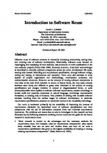
has been made in quantifying these benefits, whereby their “intangible” nature is often cited. Lacking a systematic approach to strategic value, a coherent relationship to competitive strategy is difficult to develop. Value-Based Reuse Investment Strategic Options
Operational Economics Discounted cash flow, ...
Contingent claims analysis, ... MECP framework, ... Figure 1: VBRI Framework The rest of the paper is organized as follows. We begin with a discussion of traditional discounted cash flow methods for evaluation of reuse investments. We continue with a discussion of decision tree analysis and managerial flexibility. We then introduce the application of option pricing theory, or contingent claims analysis, to reuse-related investments, particularly investments in reuse infrastructure. We conclude with a strategic framework—called Value Based Reuse Investment (VBRI)—for applying the disciplines of business strategy to investments in software reuse (Figure 1). 2. PRESENT VALUE CONCEPTS Many approaches to analyzing the economic value of investments in software reuse have been proposed in the literature. Lim [1996] has made an exceptionally thorough survey. Favaro [1996a] has compared several approaches to valuation cited in the literature on software reuse economics, including time to payback, “amortization,” and profitability index, concluding that Net Present Value (NPV) is superior to other, ad hoc approaches. Following standard texts on financial theory in this section [Brealey and Myers 1996; Trigeorgis 1996], we introduce and motivate concepts of value, risk, and decision modeling, together with illustrative scenarios. The concept of present value is an essential tool for giving proper weight to all present and future costs and benefits resulting from an investment. Based upon the simple notion that a dollar today is worth more than a dollar tomorrow (known as the “time value of money”), the Discounted Cash Flow (DCF) formula “weights” the relative contributions of cash flows that are more or less distant in the future with the application of a discount rate r according to the period (e.g. the year) in which the cash flows Ci occur. PV
=
C1 C2 + +... 1 + r (1 + r ) 2
-2-
The contribution of each cash flow Ci to the Present Value (PV) of the investment is weighted by the compounded discount rate (1+r)i. Since the cash flows are generally preceded by an initial investment C0, the Net Present Value (NPV) adds this (usually negative) cash flow NPV = C0 + PV to capture in a single number the totality of all contributions to the value of the investment. The investment decision then reduces to a single rule: make the investment if its NPV is positive. One way of looking at the discount rate r is to consider it the penalty for delay of a cash flow (like interest on a loan). Another important point of view is that of the investor, who always has alternative investments available, such as Treasury Bills (which carry no risk) or common stocks (which carry varying amounts of risk). This point of view forms a link between financial and real-world investments. The investor considers a prospective investment in a real-world project to be in “competition” with the others available to him, including those on financial markets. If one thinks of a real-world project (e.g. development of an object-oriented framework) as having a “twin security” (a financial security or portfolio of securities) with the same risk characteristics then the expected rate of return r from that security becomes the “cost of capital” for the real-world project, since the real-world project must offer a higher expected return to attract the investor’s capital—and thus, it is also the discount rate used in the DCF evaluation of the real-world project. From this point of view, DCF evaluation of a real-world project is effectively a way of analyzing what the shares of a company that carried out only that project would be worth if they were traded on the financial markets. (There are indeed many software companies whose sole business consists of a single kind of project—such as object-oriented frameworks.) As an illustration of the DCF technique, consider a scenario in which a software company has been offered a contract to create a set of CD-ROM titles for a large game-producing corporation. The corporation has guaranteed the purchase of a certain number of titles produced over a three year production schedule. In a first one-year phase, the company implements a software repository of multimedia components for an investment of one hundred thousand dollars. In a second one-year phase, it staffs the department and launches production at a cost of three million dollars. The corporation buys all of the production of the third one-year phase at a price specified in the contract of 3.5 million dollars. This contract carries no risk for the company, since its income is certain. For now, we note that this implies that it can be discounted at a risk-free rate rf, for example 5%. (Later we will expand on the topic of risk.) Using standard DCF then, the net present value (in millions of dollars) of this contract is C1 C2 + 1 + r f (1 + r f ) 2 ( −3.0) +3.5 = ( −0.1) + + 1.05 (1.05) 2 = 0.217
NPV = C0 +
At approximately $217 thousand, the positive NPV warrants accepting the contract. The Discounted Cash Flow formula, so conceptually simple, is remarkably robust in its ability to capture many important aspects of an investment decision. Short-term benefits, longterm benefits, and the investments made to achieve each can all be represented in the same formula and their respective contributions weighted over time. In other words, aside from its role -3-
in calculating the value of investments, it is a useful way of thinking about them—a theme that will recur later in this article. Over the years, DCF has become synonymous with NPV. This is not surprising, since they were essentially developed together. But in fact it is important to keep the role of each separate: • NPV represents the net totality of all contributions to the value of an investment; • DCF is a technique used in the calculation of NPV. Over the past several years the DCF technique has been criticized as not capturing some important contributions to Net Present Value [Ross 1995]. In particular, DCF has been criticized for undervaluing investments that have an important strategic component. Later on, we will argue that this is also true for many reuse-related investments, and we will explore the notion of “expanded NPV” [Trigeorgis 1996]. 2.1 Risk It is conventional wisdom that management buy-in is one of the most important prerequisites for successful reuse programs. Yet the authors have often seen managers in everyday business situations resisting buying into the strategy that has clearly been demonstrated to them to be the value-maximizing strategy. Often this hesitation turns out to be rooted in their great aversion to downside risk. Managers are well aware that reuse-related projects are likewise subject to many uncertainties. (Frakes and Fox [1996] have written at length about reuse failure modes.) Thus any reuse investment framework must deal clearly with the subject of risk. 2.2 Systematic and Unsystematic Risk It has long been accepted in financial theory that there are two kinds of risk: unique risk, which is specific to a company (or project); and market risk, which affects all companies (or projects) that participate in the economy. • Bill Gates might take early retirement from Microsoft • A component might not be reused Unique (unsystematic) risk
• Hewlett-Packard might not be able to develop a breakthrough framework technology that can be re-targeted to multiple domains • A domain analysis might fail to identify a generic architecture • inflation might increase • the budget deficit might increase
Market (systematic) risk
• Treasury bill interest rates might rise • real GNP may decline Table 1: Systematic versus Unsystematic Risk
As shown in Table 1, the risk that Bill Gates may opt for early retirement is clearly specific to Microsoft. But the risk that the Treasury may announce higher interest rates (thus causing funds to flow out of the stock market) affects all companies, regardless of what they do. Which kind of risk is more important? In fact, both play important roles, but it is important to understand the difference. In particular, it is important to understand that the company (or project) is in a different position from an outside investor. While unique risk is important to the company/project, the investor can eliminate unique risk through diversification. In fact, a well-diversified portfolio containing, say, fifteen stocks, will exhibit nearly only market or systematic risk. The basic -4-
intuition is that unique risks tend to cancel each other: the danger that Bill Gates may quit Microsoft is offset by the possibility that Hewlett-Packard may succeed in developing a new framework technology. But all companies/projects are exposed to market/systematic risk—it cannot be eliminated by diversification. Because of this, it has been observed that investors are in fact more concerned with market risk (which they cannot eliminate) than unique risk (which they can eliminate). Keeping in mind that the opportunity cost of a project reflects the return that investors expect from the project in comparison to other equally risky projects, this means that a proper treatment of risk must take systematic risk into account. 2.3 The Capital Asset Pricing Model We have noted that investors are mainly concerned with market risk. (This fact is reflected, for example, in the strong interest today in “index funds” that simply track the market.) They demand a higher return from projects with higher market risk. But how much higher? The Capital Asset Pricing Model (or CAPM) gives the answer: the return expected by investors is proportional to the stock’s/project’s sensitivity to market movements. This sensitivity is known simply as beta (β). The market (e.g. a hypothetical portfolio of all stocks) has by definition an average beta of 1.0. Technology companies (and therefore their projects, on average) tend to be high beta. (This is why we often hear phrases like “Tech stocks rise and fall the most in market swings.”) Table 2 shows some typical betas of technology companies [Brealey and Myers 1996]. Company Beta AT&T
0.92
Biogen
2.20
Compaq
1.18
Hewlett-Packard
1.65
Microsoft
1.23
Table 2: Estimated Tech Company Betas 1989-1994 For completeness we note that company betas cannot necessarily be used as-is for project betas, because company betas reflect risk on all assets, including debt. (Microsoft is an unusual case, having a policy of avoiding debt.) Debt betas (reflecting financial risk) must be factored out first to arrive at project betas (reflecting only business risk). Consistent with its role of reflecting the sensitivity of a stock to market movements, beta is generally estimated by regressing stock returns to market returns over a selected historical period. [McTaggart et. al. 1994] includes a discussion of how betas are estimated at Marakon Associates according to both historical and prospective returns. As a rule of thumb, it is difficult to arrive at a precise calculation of project betas, but it is not difficult to obtain a sufficiently close estimate for valuation purposes. 2.4 Risk-Adjusted Discount Rates Now let us return to Discounted Cash Flow and see where this discussion of risk fits in. Systematic (market) risk is accounted for in DCF calculations through the use of a higher “riskadjusted” discount rate (RADR), thus raising the “hurdle” that the project must overcome to have an NPV greater than zero. The Capital Asset Pricing Model relates this risk-adjusted rate (which we denote as k) to the risk-free rate rf through beta as follows: -5-
k
= rf + β × (rm - rf)
where rm are the returns yielded by the market as a whole. As an example, if the current expected stock market returns are 13%, against the risk-free returns of 3-month Treasury bills of 5%, then Microsoft, with a beta of 1.23 (and no company debt), could calculate its risk-adjusted discount rate as follows: k
= 5% + 1.23 × (13% - 5%) = 14%
Often, a company uses a single company-wide (or perhaps division-wide) RADR for “normal” projects. This “normal” RADR is then adjusted upward or downward for projects of higher or lower (systematic) risk. Alternatively, some companies attempt a classification of projects according to riskiness with associated discount rates, as in Table 3. Project type
Discount Rate
Pioneer technology
30%
New product introduction
20%
Existing business
15% (the “normal” rate)
Proven technology
10%
Table 3: Typical risk categories for projects Returning to the original scenario, suppose now that the software company has decided to enter the market for CD-ROM titles. In a first one-year phase, the company implements a repository of multimedia components for an investment of one hundred thousand dollars. In a second one-year phase, it staffs the department and launches production at a cost of three million dollars. Unlike the first scenario, however, where someone has guaranteed purchase of its output, the company will operate on the free market, where it has estimated annual cash flows of $700K over a seven-year time horizon, considered to be the useful life of the project. Unlike the first scenario, this project carries risk. If the company has a RADR of k = 15% for projects in this risk category, then using standard DCF, the net present value (in millions of dollars) of this project is 8
Ci i i =1 (1 + k ) ( −3.0) 8 0.7 = (−0.1) + +∑ 115 . . i i = 2 115 = -0.176
NPV = C0 + ∑
Management would be led to reject the project based on this NPV of minus $176 thousand.
-6-
2.5 Certainty Equivalent Cash Flows In the RADR approach, the denominator in the present value formula is adjusted to account for risk (and simultaneously, the time value of money). But of course, we could equivalently adjust the numerator instead, to obtain the same present value. That is, PV
=
CEQt Ct = t (1 + r f ) (1 + k ) t
thus CEQt =
Ct (1 + r f ) t (1 + k ) t
1 + rf = Ct × 1+ k
t
This adjusted cash flow CEQ is called the certainty equivalent, because it represents the equivalent certain (riskless) cash flow that would yield the same present value as the risky cash flow if there were no market risk involved (thus making is possible to discount at the risk-free rate). Viewed another way, it represents the cash flows that would yield the same present value if investors were “risk-neutral”, that is, were indifferent to market risk, and thus required only the risk-free rate of return. As an example, consider the cash flows of the last scenario, depicted in Table 4. Cash Flows (in thousands)
Risky (k = 15%)
Certainty Equivalent (rf = 5%)
C0
-100
-100
C1
-3000
-2739
C2
700
584
C3
700
533
C4
700
486
C5
700
444
C6
700
406
C7
700
370
C8
700
338
NPV
-176
-176
Table 4: Certainty Equivalent Cash Flows Note that the certainty-equivalent approach separates the treatment of (systematic) risk from the time value of money. It adjusts cash flows for risk in the numerator, and handles the time value of money in the denominator. This allows us to observe directly the fact that distant cash flows are riskier: in our example, identical cash flows of 700 are exposed to progressively more periods of systematic risk and thus decline steadily in the certainty-equivalent version. 2.6 Cash Flow Forecasts and Risk We have seen how certainty-equivalent cash flows “adjust for risk.” However, a serious misunderstanding often arises in this regard which leads project analysts astray in everyday situations. -7-
Project
Unique Risk
Market Risk
Bank Loan
None
None
Playing the national lottery
High
None
Component repository for company’s core business projects. Project leader: Thomas Edison
Low
Normal
Component repository for company’s core business projects. Project leader: Dilbert
High
Normal
Table 5: Unique versus market risk As seen in Table 5, a bank loan has neither unique nor market risk. A lottery player has a very high uncertainty of striking it rich, but his fortunes are quite independent of phenomena such as the prevailing interest rates. Note in particular the last two examples. Having a highly competent team in a particular project certainly increases the probabilities of success for that project, but from the outside investor’s point of view, the associated risk is diversifiable over his many investments—it is more important that the project is in the company’s normal line of business. Now consider the various uncertainties in reuse-related projects that may lead to success or failure. • • • •
Will the domain analysis succeed in identifying a generic architecture? Will we succeed in reengineering the system? Will we find enough components to populate the repository? Are our programmers competent enough to apply this new technology (e.g. Object-oriented patterns) for developing the reuse repository?
Certainly, all of these uncertainties introduce risk into reuse projects—they make the project’s outcome less certain—and they must be accounted for when evaluating prospective investments. But there is a right way and a wrong way to do this. Project analysts are often tempted to simply raise the discount rate—say, from 15% to 20%—when they perceive the project’s outcome as less certain. In this way, they feel that they have “accounted for the extra risk.” But the discount rate is really intended to model systematic risk, and for most practical applications it can and should be provided to the analyst by his company. In another approach, the analyst might try adjusting cash flows downward and then discounting at the risk-free rate, in the style of certainty equivalents. This approach is also incorrect, and reveals a misunderstanding about the nature of project-specific versus systematic risk. As a specific example, Malan and Wentzel [1993] propose that cash flows associated with future reuse of a component (the “good” outcome) be multiplied with a probability p reflecting the possibility that the reuse instance might not be actualized (the “bad” outcome). Are these probabilities some kind of certainty equivalence adjustment as seen in the previous section? Can the risk-free discount rate now be used? No: certainty equivalents deal with systematic risk. The uncertainties we usually deal with (such as those listed above) are really project-specific risks, and have to do with making good cash flow forecasts. Malan and Wentzel are describing how to arrive at unbiased cash flow forecasts. (Unbiased cash flow forecasts will tend to be accurate over the long run.) If a forecast cash flow is unbiased, then it tries to account for all possible outcomes, good and bad. As Malan and Wentzel suggest, many techniques for assisting in resolving
-8-
uncertainties in cash flow forecasts are now available, such as sensitivity analysis and simulation. In summary, therefore: 1. Deal with unique, project-specific risk through unbiased cash flow estimates that consider all possible outcomes, both good and bad; 2. Deal with systematic, market risk by estimating project beta (or obtaining it from your company’s treasury) and applying a risk-adjusted discount rate or certainty equivalent cash flows (especially when different discount factors must be used in different periods). For a project analyst, the greatest challenge is in making good cash flow forecasts. These forecasts are associated with the project’s unique risk—and it is important to keep them that way by not “hiding” uncertainties in an artificially inflated (or deflated) discount rate. 2.7 Observations on DCF Techniques Before continuing, let us summarize the discussion so far. With NPV established as a foundation for valuation, we have seen that discounted cash flow provides a robust method for capturing the value over time of many of the operational benefits and costs associated with reuse investments. With the help of a broad palette of reuse metrics [Poulin 1997a], these costs and benefits—for example, short-term increased labor costs and long-term reduced maintenance costs—can be estimated, and combined into a single, unified estimate of value. We have also seen that DCF techniques can deal with both project-specific risk (through unbiased expected cash flow forecasts) and systematic risk (through application of the CAPM) associated with these operational costs and benefits. These techniques are mature, well-understood, and well-accepted in the business community. DCF techniques can be used to evaluate the operational benefits from “business as usual” (and this is often the case in a stable, well-developed program of systematic reuse with wellunderstood and measurable costs and benefits). But as valuable as these operational benefits are, they don’t do justice to the full value of reuse. When we begin to speak in terms of other contributions to business value such as “flexibility” or “strategic opportunities,” DCF techniques have little to offer us. More powerful techniques are needed. 2.8 Decision Tree Analysis and Active Management Discounted cash flow techniques were originally developed for the valuation of financial instruments such as stocks, bonds, and savings accounts. Such instruments are passive in nature— there is little one can do to change the behavior of a savings bond. But in the real world the manager has choices. He can intervene to change his strategy when circumstances warrant it. Decision Tree Analysis (DTA) was developed to model the different kinds of outcomes and management decisions that can occur in the real world. Clemons [1991] shows an example of DTA applied to a strategic IT investment scenario. Let us now consider a more realistic scenario for our CD-ROM example, modeling the points at which management can make choices. In a preparatory step, the company commits a small team at a cost of one hundred thousand dollars to study the technology and develop a baseline repository of software multimedia components. If that step goes well, then the company will commit to enter the CD-ROM marketplace and build up a department, at a cost of three million dollars. In the uncertain environment, the planners can imagine three general levels of success in the market: high, medium, or low. The decision tree for this scenario is shown in Figure 2. -9-
Start Launch repository project (invest $100K)
no
Repository populated
no
30%
70%
Year 1 Launch commercial venture (invest $3M)
no
Year 2 Low (20%)
Year 3
-$0.1m
High (20%) Medium 60%) $4m
$8m
Figure 2: Decision tree representation of multimedia venture There are two kinds of nodes in this decision tree: • outcome nodes (circles), where uncertainty is resolved by events and observed by management. The success of the repository initiative, and the market acceptance of the commercial venture are nodes of this type; • decision nodes (squares), where management has the opportunity to intervene actively. The initial decision to build the repository, and the subsequent decision to launch the commercial venture are nodes of this type. Effectively, it is a game where management makes each move in response to the move of its counterpart (e.g. competition, the market, nature). Note that later events in the decision tree are conditioned by earlier events (i.e. the various market success probabilities of the CD-ROM venture are conditioned by success in creating the repository.) Thus present values are calculated in a roll-back, dynamic programming fashion by moving backwards from the final outcomes to the beginning. Suppose the company’s risk-adjusted discount rate is k = 10%. The expected present value in the final year of the scenario for all future years is given by the projected cash flows weighted by their probabilities. PV3 = (0.2)(-0.1) + (0.6)(4) + (0.2)(8) = 3.98 Moving back one year and discounting at a cost of capital of 10%, we obtain PV2 = PV3 / (1+k) = 3.98 / 1.10 = 3.6 This is therefore the present value of expected future cash flows when the CD-ROM department has been created and the venture goes to market. - 10 -
Moving back one year to the creation of the commercial venture, the investment of three million dollars is accounted for in the present value calculation: PV1 = PV2 / (1+k) - (Investment1) = 3.6 / 1.10 - 3 = 0.27 Moving back one more year to the original decision to start the multimedia repository initiative, we weight once again the expected values of the two possible outcomes by their probabilities, discount back once again, and subtract the original hundred-thousand dollar investment. PV0 = PV1 / (1+k) - (Investment0) (0.3)(0.27) + (0.7)(0) = − 0.1 110 . = -0.026 At minus $26 thousand, the negative NPV of this scenario would discourage the decision to invest. 2.9 Problems with Decision Tree Analysis Decision Tree Analysis helps overcome the major failings of DCF, which treats real projects as passive investments, by making it possible to model project outcomes and management intervention explicitly. The ability to model the choices available to management is absolutely critical to a realistic assessment of the value of a reuse project. But in practice, decision trees have proven to be unwieldy, growing wildly into “decision forests” as the number of choices grows. This characteristic has impeded their use in many situations. But the real problem with decision trees lies elsewhere: in its treatment of risk. In our example, a single discount rate was used throughout the entire decision tree. Was that realistic? Surely not: as uncertainty was resolved and management intervened to make choices, the project itself changed its nature over successive sequential investments—from pioneering technology to “normal business.” Risk was clearly affected, and so a single discount rate is no longer applicable. We could try to introduce multiple discount rates. However, aside from the practical difficulty of doing this, we will see later that there are fundamental theoretical problems with the treatment of risk in traditional DTA. Thus the traditional tools of DCF and DTA bring us to a dead end when we want to go beyond the analysis of operational characteristics of projects. For this reason, we now move beyond these traditional tools and explore a more powerful set of economic modeling techniques. 3. FINANCIAL AND REAL OPTIONS In the real world of project management, we often talk about “creating options,” or “keeping our options open.” There is a growing community that now believes that option pricing theory in fact provides the most valid and rigorous foundation upon which to build a framework for capturing strategic value. Option pricing theory has also given us a way to deal with several thorny issues in the treatment of risk and active management that DCF and DTA have proven unable to handle. In this section we provide a relatively self-contained introduction to options and the most important techniques for evaluating them arising from option pricing theory [Brealey and Myers 1996; Trigeorgis 1996]. This approach to valuation is known as contingent claims analysis (CCA). - 11 -
3.1 Introduction to Options The Chicago Board Options Exchange (CBOE) was created in 1973, the same year that a rigorous pricing formula for options was finally discovered by Black and Scholes [1973], ending a search by economists that had lasted for decades. (Scholes and his colleague Merton were awarded the Nobel Prize in Economics in 1997 for their pioneering work in option pricing theory.) Today, options are traded all over the world on assets ranging from common stocks and bonds to commodities, foreign currencies, and stock indexes. Options owe their usefulness to their essential asymmetric property: the right—without an associated obligation—to buy or sell an asset. (Futures contracts, in contrast, are symmetric, with an associated obligation to buy or sell.) It is this property that will ultimately make it possible to model essential characteristics of reuse investment that are not captured by traditional methods. In this initial overview of options, we will confine ourselves to financial assets. Later, we will map the concepts onto a real-world context. A call option is the right to buy an asset at a specified time in the future for a specified exercise or strike price. A put option is the right to sell an asset in a comparable manner. A European option may be exercised only on the date specified. An American option may be exercised at any time up to the date specified. (European and American call options have the same value in the absence of dividends—Microsoft, for example, has never paid a dividend—because a call option is more valuable “alive” than exercised, and therefore it would not pay to exercise the American option early. But if the underlying asset pays dividends, then it may be worthwhile to exercise an American option early in order to capture the dividend cash flows.) As a simple illustration of these concepts, imagine a dynamic young reuse consulting company Reuze, Inc. which has recently had a successful initial public offering. The position diagram in Figure 3 illustrates the values of a call and a put option written (sold) on Reuze stock for an exercise price of 50 dollars. Value of call
Value of put
50
50
50
Share price
50
Share price
Figure 3: Position diagrams for call and put on Reuze, Inc. The call option’s value at expiration is worthless unless the price of Reuze stock has risen above the exercise price. After that, it increases in lock step with the share price. Conversely, at expiration, the put option is worth its full value at an underlying share price of zero, decreasing and finally becoming worthless as the share price rises above the exercise price. (This “floor” is what makes put options especially useful as hedges.) As illustrated above, it is easy to determine the value of an option at expiration—once it is acquired. But what eluded financial economists for decades was the price that the purchaser should pay to acquire the option.
- 12 -
3.2 Pricing By Replicating Portfolio The great breakthrough by Black and Scholes in their landmark publication in 1973 was the insight that for a given option on a given stock, it was possible to construct a replicating portfolio containing a mixture of shares of that stock and a loan (at normal risk-free interest rates), in such a way that the expected returns on that portfolio were exactly the same (“replicating”) as the expected returns on the option. The basic idea behind the construction of this replicating portfolio can be illustrated with the scenario depicted in Figure 4, in which a stock is held for one period of time (e.g. six months), and at the end of that period will have either risen according to a multiplicative parameter u with probability q, or fallen according to a multiplicative parameter d with probability 1-q. (In practice these multiplicative factors are generally derived from the variance of the stock price.) Pu = P × u
q P 1-q
Pd = P × d
t0
t1 Figure 4: Single Period Stock Behavior
As a concrete example, suppose that our dynamic young company Reuze is currently trading at 50 dollars, and after a single six-month period will have either risen 25 dollars to 75 (u = 1.5), or fallen 15 dollars to 35 (d = 0.7). Suppose also that there is an equal probability of a rise or fall in the stock price (q = 50%). A call option written for an exercise price of 45 dollars would be worth either Cu = $75-$45 = $30 if the stock rises, or Cd = $0 if the stock falls (since exercising the option for $45 would result in a loss). Now let us replicate the behavior of this call option with a suitably constructed portfolio. Suppose the prevailing interest rate on six-month bank loans is 3%. We buy exactly 3/4 of one share of Reuze, financing part of the purchase with a six-month bank loan of exactly $25.49. Now let us look at the returns we can expect from this mixed holding of stock and borrowed cash. First of all, the loan will have to be repaid with interest after six months. This repayment amounts to $25.49×1.03=$26.25. Subtracting the repayment from the value of the holding in Reuze stock, we obtain the expected returns shown in Table 6. Portfolio return at end of period
If price rises to $75
If price falls to $35
Value of 3/4 share of Reuze
$56.25
$26.25
Minus loan repayment with interest
- $26.25
- $26.25
Portfolio Value
$30.00
$0.00
Table 6: Returns on replicating portfolio of Reuze shares Thus, our portfolio exactly “mimics” the behavior of the Reuze call option. The price of this portfolio was simply what we had to pay to make up the difference between the cost of the 3/4 share of Reuze and the bank loan we took out: C
= 3/4 × $50 - $25.49 - 13 -
= $12.01 This is where we now make use of the “no arbitrage” principle of efficient markets: since the call option has exactly the same expected returns as the replicating portfolio, then it must have the same price. Otherwise, a clever investor could take advantage of the arbitrage opportunity created by the price difference to create an infinite cycle of “buying low and selling high”—in other words, a perpetual “money machine.” Thus, in general we can state the following: C ≈ where C = N = P = L =
N×P - L value/price of the call option number of shares of the stock to buy price of the stock value of the loan in dollars
The number N of shares to buy is given by the ratio of “spreads” of the option and the underlying share prices. (This ratio is known as the option delta). N
=
Cu − Cd Pu − Pd
In our Reuze example, 3/4 of one share was purchased. The amount of the loan is simply the difference between the payoff from the N shares purchased and the payoff from the option (discounted back to a present value at the risk-free interest rate). L
=
N × Pd − Cd 1 + rf
In our example with Reuze stock, the amount of this loan was $25.49. 3.3 Risk-Neutral Option Valuation Now let us bring the subject of risk back into the discussion. Something peculiar can be observed about the calculations of the previous section: it was never mentioned whether Reuze was a high-beta “high-flyer” or low-beta “blue chip” stock—as though its systematic risk didn’t even matter. In addition, the probability q of a rise in the stock price did not affect the result at all. Return at end of period
If price rises to $75
If price falls to $35
Value of 3/4 share of Reuze
$56.25
$26.25
Minus (possibly) exercised call option
-$30 (option exercised at $45)
-$0.00 (option not exercised)
$26.25
$26.25
Portfolio Value
Table 7: Hedged portfolio of Reuze shares Let us dwell a bit on this surprising observation. Consider again the call option on Reuze stock that was priced in the previous section. Suppose that, instead of the buy-and-borrow - 14 -
scenario described above, we had bought 3/4 share of Reuze without borrowing, and sold that call option (with exercise price of $45) to some other investor. The price of this portfolio would be 3/4 × $50 - $12.01 = $25.49. Table 7 shows the expected returns on the portfolio. Thus, this strategy guarantees a fixed return at the risk-free rate no matter what happens to the price of Reuse stock; and furthermore, regardless of the discount rate associated with Reuze stock. We have “hedged our bets” and completely eliminated the risk from this portfolio. (In effect, this portfolio behaves like a bond.) The option delta presented in the previous section is also known as the hedge ratio. The reason for this name is that options make it possible to “hedge,” that is, to construct a portfolio that yields a risk-free return through a combination of buying securities and selling options which effectively “cancel out” each other’s risk and yield a risk-free return. This is true in “all worlds”— that is, regardless of investors’ attitudes towards risk. This important property suggests a simpler and more convenient way of pricing options: for purposes of the valuation, simply assume a riskfree world. In such a risk-neutral world, all assets (stocks, bonds, options, bank loans) would earn the same expected return—the risk-free rate. In the case of Reuze stock, we know that its real return will be either Ru = u-1 = 50% if it rises, or Rd = d-1 = -30% if it falls. These two possible returns would be weighted by their equal probability of occurrence (q = 50%) to yield its expected return, corresponding to a risk-adjusted discount rate of 10%. = q × Ru + (1 − q ) × Rd = 50% × 50% + 50% × (−30%) = 10%
k
But the expected return on Reuze stock in a risk-neutral world would be only 3%, the risk-free rate, so these real returns must be weighted by appropriate hypothetical probabilities p and 1-p of their occurrence. The hypothetical “risk-neutral probability” is simply calculated as = p × Ru + (1 − p) × Rd
rf
Thus, p
=
(r f − Rd ) ( Ru − Rd )
In our example, p
=
3% − (−30%) = 41.25% 50% − (−30%)
Now that we know the probabilities of rise and fall of Reuze stock in this hypothetical world, it is a simple matter to calculate the expected returns on the call option (since, as a derivative, it depends on the stock). Remembering that the option will be worth either $30 if Reuze rises, or nothing if Reuze falls, the expected value of the option at the end of the period is C1
= (41.25%) × ($30) + (58.75%) × ($0) = $12.38
In this hypothetical risk-neutral world we can obtain the initial value of the call option (and therefore its price) by discounting back at the risk-free rate: - 15 -
C0
= C1 / (1 + r f ) = $12.38 / (1.03) = $12.01
This is exactly the same result as given by the replicating portfolio approach. The risk-neutral approach is an important application of the certainty equivalents concept that was introduced in Section 2.5. The substitution of hypothetical cash flows for “real” cash flows in the certainty-equivalent calculation of NPV make it possible to use the risk-free discount rate. Similarly, the substitution of hypothetical transition probabilities for “real” transition probabilities in risk-neutral option valuation make it possible to use the risk-free discount rate. It allows us to finesse the extremely thorny problem of the fluctuating systematic risk of options. We will present an example of risk-neutral valuation in Section 4.3, in the context of evaluating flexibility in reuse infrastructure investments. 3.4 The Black-Scholes Formula Clearly it is not very realistic to expect only two possible share prices (“up” and “down”) at the end of a period. It would be better to chop up the period into as many intervals as possible (e.g. a month, a week, even a day), increasing the range of possible values and providing a more realistic distribution of returns. This generalized technique is the discrete multiplicative binomial method [Cox et. al. 1979]. As the number of intervals increases, the binomial method converges in its continuous limit to the famous formula first developed by Black and Scholes. C = [ N (d1 ) × P] − [ N ( d 2 ) × PV( EX )] where log[ P / PV( EX )] σ t d1 = + 2 σ t d2 = d1 − σ t N(d) = cumulative normal probability density function EX = exercise price, whereby the present value PV of the exercise price is obtained by discounting back by the (continuously compounded) risk-free interest rate t = time to exercise date of option P = price of security σ = standard deviation per period of continuously compounded rate of return on security. (The above is the original formulation, which is valid only for call options on nondividend-paying stock. Extensions exist for valuing call options on dividend-paying stock [Chriss 1997].) The Black-Scholes formula gives an elegant closed-form solution to many useful option valuation problems, and makes it possible to obtain an intuitive feeling for the behavior of the option’s value as a function of its parameters. 1. The stock price itself. The value of a call option on a stock must be less than the price of the stock, since a call option is, after all, nothing more than the right to buy the stock. (It would be nonsensical to pay more than the price of the stock for the right to buy the stock!) Conversely, a call option will always be worth something as long as the underlying stock price is positive— because there is at least some chance that the stock price will rise. If a stock’s price sinks to zero, then this indicates that there is no chance that the stock—and therefore the option—will ever be - 16 -
worth something in the future. The higher the stock price, the greater the chance it will exceed the exercise price of the option. 2. The risk-free interest rate. It may seem odd that the risk-free interest rate (rather than some risk-adjusted rate) would play a role in an option’s price. Consider, however, that buying an option is like buying a stock in installments, with a down payment at purchase of the option, and delayed payment at exercise time. The higher the prevailing interest rates, the more valuable the ability to delay payment becomes. 3. Stock price volatility. It may likewise seem odd that an option on a wildly fluctuating stock is more valuable than an option on a stock whose price is stable. The reason is simply that options eliminate the downside risk associated with stock fluctuations. Thus, the greater the range of possible stock prices, the greater the chances for a great deal at option expiration. 4. Time to expiration. The points mentioned above make it evident why a longer time to expiration makes an option more valuable. When viewed as a kind of stock purchase in installments, a longer time to the final payment (exercise) increases the time during which interest did not have to be paid. In addition, a longer time to expiration increases the volatility of the price, because the longer fluctuation period increases the possible number of future prices. A particularly thorough treatment of the Black-Scholes formula can be found in [Chriss 1997]. An example of using the Black-Scholes formula is illustrated later in the valuation of growth options created by reuse infrastructure investments. 3.5 Why Option Pricing Theory Is Necessary It is reasonable to ask why a special theory should be necessary for pricing options. Why isn’t discounted cash flow usable in this case? In fact, it is perfectly feasible to contemplate the calculation of expected cash flows from an option. But as we have already noted earlier in our discussion of decision trees, the real problem lies somewhere else: in the discount rate. We hinted earlier at a fundamental problem with determining the proper discount rate in decision trees. Now we know the source of the problem: decision trees have options embedded in them. An option is a derivative, whose value depends on the value of the underlying asset. As such, the risk of the option changes constantly as the price of the underlying security changes. The risk of the option also varies with time. Thus the risk is a “moving target”, and when options are present a single discount rate won’t work. Projects that have options embedded in them—thus exhibiting managerial flexibility—must be analyzed with option pricing theory (contingent claims analysis). As will be illustrated in the next section and in Section 4.3 in the context of reuse infrastructure investment, CCA is operationally the same as DTA in the sense that a decision tree is constructed; but it a risk-neutral or “certainty equivalent” decision tree, which handles the derivative nature of options correctly. CCA may thus be seen as an “economically corrected” version of DTA. 3.6 Real Options The decision tree analysis presented in Section 2.8 illustrated a situation in which management had the choice to stop the CD-ROM project if the multimedia component repository was not successfully constructed. This is only one example of the managerial flexibility that is exhibited in many (if not most) real-world projects. Once begun, projects do not need to proceed inexorably with the procedure planned at the outset. Managers can monitor the progress of projects and intervene in many to change their behavior and outcomes: • If a project is going badly, then a manager can stop it. • If prospects are good, a project can be expanded to take advantage of the good conditions. - 17 -
• A manager can reallocate resources in a different way according to varying requirements. • If a manager is not sure about the prospects for a project, he can wait to start it. For example, if it is not certain that a new technology will catch on, then the manager can wait a year or two before investing. It has been recognized that these examples of managerial flexibility can be thought of as real-world versions of the same options that are seen in financial markets—that is, as “real” options (as opposed to “financial” options). This insight has made it possible to bring the power of options pricing theory to the modeling and analysis of the options that are embedded in real-world projects. Trigeorgis [1988] illustrates the analogy as shown in Table 8. Call option on stock
Real option on project
Current value of stock
Gross present value of expected cash flows
Exercise price
Investment cost
Time to expiration
Time until opportunity disappears
Stock value uncertainty
Project value uncertainty
Risk-free interest rate
Risk-free interest rate Table 8: Financial/real option analogy
Some of the earliest applications of the real options approach were in natural resource investments (such as oil reserves or gold mines). In addition, the approach has been applied in several industries, including pharmaceutical development, real estate, insurance, leasing, manufacturing, and shipping. [Trigeorgis 1996] contains an overview. Of particular relevance in our context is the option value of information technology infrastructure investments, which has been a subject of study for several years [Dos Santos 1991]. Clemons [1991] refers to the concept in an informal way when describing strategic IT investments as “strategic options on the future of the enterprise.” In particular, an ongoing effort at Boston University by Henderson [Moad 1995] and more recently his colleague Kulatilaka has the goal of integrating options approaches into maximizing value in IT infrastructure capability. Flatto [1996] gives an overview of many kinds of options in information technology investments. 3.7 Is the Analogy Justified? Several conceptual objections have been raised concerning the validity of carrying over the theory of contingent claims analysis into a real-world context. We cover the most important ones in this section. Traded versus non-traded assets. As we have seen earlier, the central concept in the pricing of options is the replicating portfolio of financial assets, whereby the trading opportunities of investors on the markets eliminate arbitrage opportunities. But real-world projects (e.g. developing a reusable component library) are generally not traded. In view of this fact, can the analogy be justified? Mason and Merton [1985] argue that the analogy is valid if we make the same assumptions upon which Discounted Cash Flow techniques rest. As we saw earlier, traditional DCF techniques postulate a “twin” financial security (or dynamic portfolio of securities) with the same risk characteristics as the real-world project, then use a market equilibrium model such as the Capital Asset Pricing Model to determine its sensitivity to market movements and estimate its required rate of return (discount rate). A (non-traded) real option on the real-world project can be valued with the same reasoning by linking it to the value of the (traded) option on its twin - 18 -
security. Consistent with the approach of contingent claims analysis, we will make use of the “twin security” assumption in our application of option pricing formulas to real-world projects. Contingent claims analysis assumes a particular model of the stochastic process that underlies the movement of stock prices in time. The geometric Brownian motion model is generally used to describe the probability distribution of future returns on stocks. Thus the application of the “twin security assumption” implies the acceptance of this model for the movement in time of the value of the underlying real asset in a real-world project. McDonald and Siegel [1984] discuss some of the issues in applying this model to nontraded real-world projects. Interestingly, even the geometric Brownian motion model of stock price movements has not been free from criticism. There is empirical evidence that this model seriously underestimates the probability of large drops in the market—indeed, Jackwerth and Rubinstein [1995] observed that under the assumptions of this model, the great crash of 1987 was effectively impossible. Shared Ownership of Real Options. A call option on a stock is the sole property of its owner, who may exercise it at his discretion. That is, he has no “competitors.” Some real options, such as patents on certain kinds of technologies, are effectively proprietary. But especially in the software industry, many options are effectively opportunities that are shared by all competitors. One need only consider the introduction of the Java programming language by Sun Microsystems and its enthusiastic adoption by many competitors [IBM 1997] as part of their own competitive strategies. The very introduction of the technology made it in a sense “shared by all.” Similar arguments can be made concerning object-oriented framework technology. Of course, the competitive position of a firm may be such that its options become effectively proprietary. It would be difficult to argue that any firm except Microsoft currently has a real option to develop a successor to its suite of office automation products. Competition and Preemptive Exercise. The fact that many real options (including many in the software industry) are not traded and effectively shared by many competitors can change the optimal exercise policy that would exist for a traded financial option. For example, Sullivan et. al. [1997] discuss software design decisions in the context of an option to delay investment in the face of uncertainty surrounding questions such as the future availability of better software restructuring tools. The presence of competition may force the investment to be undertaken earlier than otherwise would have been optimal, in order to preempt the competition from exercising its shared option [Dixit 1980]. Consider the rush to implement new Internet technologies when they are still immature in order to be “in the game.” Indeed, game-theoretic approaches are currently being integrated into real options theory in this context [Smit and Ankum 1993]. Competitive preemption, of course, is the rationale behind much of the current focus on time to market in the software industry [Jacobson et. al. 1997]. Malan and Wentzel [1993] have analyzed the value of reduced time to market in terms of traditional Discounted Cash Flow. However, since the benefits sought tend to be more strategic than operational, the options and game-theoretic approaches mentioned above are a more promising avenue for exploring this kind of issue. Multiple, interdependent real options. The value of a financial option when exercised depends only on the underlying financial asset. In the real world the situation is rarely so simple. Exercising a real option (e.g. investment in a component repository) may well yield another real option (e.g. further investment opportunities), in a chain of interrelated investments, perhaps including intermediate competitive reactions. Moreover, real-world scenarios often contain multiple, interacting real options, whose analysis leads to serious problems of computational complexity [Trigeorgis 1991]. Forecasts of option parameters. The valuation of options involves the estimation of the behavior of several parameters, ranging from exercise price to the distribution and variance of the future option value. For financial options, there are several proxies available to predict this - 19 -
behavior—the most obvious proxy is simply historical values of a financial asset. In real options such proxies rarely exist, and the analyst must rely on experience and judgment in his estimations. We will return to these considerations in the context of the concrete examples presented in the next section. 4. STRATEGIC OPTIONS IN SOFTWARE REUSE INVESTMENT In this section we examine how the techniques of contingent claims analysis can be applied to model strategic sources of value associated with software reuse investments. 4.1 Reuse Infrastructure Investments In [Karlsson 1995] a useful distinction between development for reuse and development with reuse is made. Increasingly, development for reuse is viewed in the context of an overall investment in reuse infrastructure. An example is the kit concept [Griss and Wentzel 1994], whereby the reuse infrastructure includes not only reusable components and frameworks, but also glue languages, generators, test suites, documentation, and other support technology. An even broader perspective is taken by Jacobson et. al. [1997] in the Reuse-Driven Software Engineering Business, whereby the enterprise is encouraged to “invest in and continuously improve [technological] infrastructure, reuse education, and skills.” In that view, the reuse infrastructure consists not only of technology (components, frameworks, languages, tools, etc., which may be developed or purchased), but also human resources (trained personnel) and organizational resources (including systematic processes). The reuse infrastructure is a large-scale investment to enable the enterprise to exploit development with reuse in pursuing its business interests. Although part of the investment in this reuse infrastructure can often be justified in terms of directly observable cash flows linked to operational benefits (such as lower subsequent production costs), intangible “strategic” benefits are increasingly being cited to justify the investment. In reuse infrastructure investment, typical strategic rationales are: • a reuse infrastructure will provide new market entry opportunities for the firm; • a reuse infrastructure will improve the firm’s agility in an uncertain marketplace. These strategic benefits are not easily quantifiable in terms of cash flows. However, the large body of work studying the option value of information technology infrastructure investments, discussed in Section 3.6, can shed light on the valuation of these benefits. 4.2 The Value of New Market Opportunities In the decision tree analysis of the CD-ROM production facility we calculated a negative NPV, discouraging investment in that reuse project. This scenario illustrates the classic problem in obtaining up-front management buy-in for reuse investments [Griss et. al. 1994]. The heart of the problem is that the true business value of many reuse infrastructure investments lies in the opportunities they open up for the investor. Let us now approach the problem from an options perspective. Consider a large European telecommunications company that would like to start a venture named TeleFrame. Its mandate is to develop object-oriented framework technology infrastructure, including associated capabilities (trained personnel, documentation, process) that will allow entry into the emerging market for value-added call services. It is only known that this market might be enormous, or might be a complete bust. If TeleFrame succeeds and the market for call services - 20 -
materializes, a new venture named RapidCall will be launched to provide large organizations with rapid customized call service creation (such as call routing, private numbering plans, FreePhone, etc. [Ku 1993]). The expected net cash flows from the TeleFrame and RapidCall ventures are shown in Table 9, together with cumulative Net Present Values. Period
Tele-Frame Cash Flows
Tele-Frame NPV in Year 0 at 20%
Rapid-Call Cash Flows
Rapid-Call NPV in Year 4 at 20%
C0
-500
-500
C1
100
-416
C2
200
-278
C3
300
-104
C4
100
-56
-1500
-1500
C5
300
-1250
C6
600
-833
C7
900
-312
C8
300
-168
Table 9: TeleFrame and RapidCall expected cash flows TeleFrame will require an initial investment of $500 Million, and will run for four years, with some cash inflows due to consulting and project work. The RapidCall venture will begin in the fourth year and run for four more years. It will be an extensive undertaking, requiring triple the earlier investment. The cash inflows from RapidCall are likewise estimated to triple in size. Unfortunately, the TeleFrame venture is expected to lose money, with an NPV of -$56 Million. By itself, it would clearly not be considered a worthwhile venture. The outlook is no better for RapidCall. A best estimate for its NPV yields a miserable -$168 Million, triple the loss of the TeleFrame venture. Since this corresponds to the NPV at the start of the RapidCall venture in Year 4, discounting back four more years yields a RapidCall NPV of -$81 Million at Year 0. Thus, if the commitment were made in Year 0 to carry through both projects, the total combined value would be NPV = NPV(TeleFrame) + NPV(RapidCall) = (-$56) + (-$81) = -$137 Million Under normal DCF rules, management would never invest in such a “losing” venture, in spite of its obvious strategic importance. But an options-oriented approach to valuation of this scenario can offer a different perspective: • The main purpose of the TeleFrame venture is to create the opportunity to invest in the RapidCall venture. Without the existence of TeleFrame, RapidCall cannot be launched. • Management has no obligation to launch the RapidCall venture if the market hasn’t developed or the framework technology hasn’t proven itself. • The prospects for RapidCall are highly uncertain. Although management has made its best estimate of RapidCall’s cash flows, the market could in fact explode—or bust. The - 21 -
TeleFrame technology is also highly uncertain. But the TeleFrame technology will be either proven or not. By Year 4, the picture will be much clearer. This reasoning reveals that the TeleFrame venture actually provides us, in addition to its cash flows, a valuable strategic growth option [Brealey and Myers 1996], the opportunity to create the RapidCall venture. In order for the true business value of the venture to be reflected, the value of this strategic option must also be represented in its NPV. This growth option is analogous to a European call option, where the “time to expiration” is the time to launch of the RapidCall venture; the “exercise price” is the investment required in RapidCall; and the “value of the underlying real asset” is the present value (from the vantage point of Year 0) of RapidCall’s projected cash flows. We can evaluate this simple option with the Black-Scholes formula. The present value in Year 4 of RapidCall’s projected cash flows (that is, excluding the $1500M investment from the NPV of -$168K) is $1332M. In order to calculate the Year 0 value of this figure, we discount the Year 4 value back to Year 0 at 20% (continuously compounded) as required by Black-Scholes. We assume that the value of cash flows from the RapidCall venture will evolve in time according to the same process as the price of a “twin security,” with a high yearly standard deviation on returns of 35%, given the high uncertainty associated with the RapidCall venture. (We will return to this assumption in the next section.) Finally, assuming a risk-free interest rate of 10%, we have all of the parameters needed for the Black-Scholes Calculation. P t EX rf σ
= = = = = =
($1332M) × e-(20%×4 years) $598.5M 4 years $1500 Million 10% 35%
Application of the Black-Scholes formula yields C
= $70M
This is an estimate of the value of the growth option provide by the TeleFrame initiative to launch the RapidCall venture four years later. Thus, the total NPV of the TeleFrame project is: NPV = (TeleFrame value) + (value of growth option) = (-$56M) + $70M = $14 million So in fact, the valuable strategic opportunity provided by the TeleFrame venture is reflected in an overall positive NPV. It may seem strange and non-intuitive to see a positive NPV on two sequential ventures, each of which has a negative NPV when taken individually. Recall, however, that the uncertainty associated with RapidCall is very high. If the market explodes and the upside of this uncertainty is realized, then RapidCall will be a big winner. If the downside occurs, then management is protected: it has no obligation to launch RapidCall. That is the essential intuition that reveals the significance of the strategic option.
- 22 -
4.2.1 Conceptual and Practical Issues Recall from the discussion in Section 3.7 that the Black-Scholes formula was developed for the evaluation of options on assets that are traded on financial markets. The RapidCall venture is not even in existence during the first three years, much less traded—thus violating a fundamental assumption of the formula. In our example we exploited the concept of a “twin security” discussed earlier. We hypothesized the existence of a stock (or portfolio of stocks) with the same risk characteristics as the RapidCall venture—and therefore an option on this (perhaps hypothetical) stock would have the same value as the option on RapidCall. Thus, we have “finessed” the problem of specifying the stochastic process underlying the evolution of the value of RapidCall’s cash flows—with a relatively strong assumption, however. Even so, the practical problem of estimating the standard deviation remains, and there is no historical data on RapidCall’s returns. Here, historical data of the stocks of companies with similar characteristics is often used as a proxy. In the high-tech industry, standard deviations of 35% or higher are not uncommon. Another problem is that the Black-Scholes formula assumes a single, constant standard deviation (in our case, 35%). It may not be realistic to make this assumption in the case of RapidCall. The elegance and simplicity of the Black-Scholes formula in its application to growth options are compelling, but it rests upon a series of assumptions that must be accounted for in its application to real-world situations. As one final example, recall that an investment in framework technology such as the TeleFrame venture involves to some degree a “non-proprietary” real option, in the sense that the competition may have similar investment opportunities. The issues concerning competitive interaction were also discussed in Section 3.7. 4.2.2 Staged Investments in Reuse The Teleframe/RapidCall initiative is an example of a staged reuse investment. For deeper insight into the option value of staged reuse investments let us return yet again to the concept of uncertainty from an options perspective. From this point of view, it is useful to distinguish two kinds of uncertainty: • economic uncertainty (such as the future health of the CD-ROM market); • technical uncertainty (such as the outcome of a domain analysis) Economic uncertainty is external—the only way to resolve it is to wait. It is often optimal to delay investment in the presence of economic risk (for example, for investments in natural resources such as oil fields [Dixit and Pindyck 1994]). Technical uncertainty, however, is internal, in the sense that we can manage and resolve it by “doing the work” and seeing the results. Contingent claims analysis can often show that it is optimal to start investment in the presence of technical uncertainty if it can be structured in a step-by-step fashion. The nature of many reuse investment opportunities is high initial technical uncertainty (for example, domain analysis, component development) which is resolved in stages, progressively reducing the variance of the uncertainty and revising expected value upward. The option value of staged investments in software development is also discussed by Sullivan et. al. [1997], whereby the analogy to some popular iterative prototyping software lifecycle models is also noted; and Withey [1996], where the development of a generic architecture is modeled as a preliminary stage to the creation of a product line business. In Decision Tree Analysis we have seen that there are major issues in dealing with the fluctuating uncertainty associated with staged investments (i.e. discounting within decision trees). See [Withey 1996] for an example and discussion of these issues. - 23 -
4.3 The Value of Flexibility The underlying economic rationale for large-scale reuse infrastructure investment can often be expressed succinctly in a single word: flexibility. We reason that by making the extra investment in a flexible development infrastructure, we will increase the agility of the firm in the marketplace. But how do we put a value on something as intangible as flexibility? The study of flexible manufacturing systems [Kulatilaka 1988] can provide useful perspectives on flexibility in the software engineering domain. Trigeorgis [1996] introduces the notion of the adaptive firm in applying the principles underlying flexible manufacturing systems to the strategic operating capabilities of an enterprise endowed with flexible technical, human and organizational resources. In this section we consider this notion in the context of infrastructure investment for development with reuse. Along the way we will illustrate the use of risk-neutral techniques to evaluate both Net Present Value and a combination of real options. The IBM San Francisco Project is an initiative to provide “application developers with a base set of object oriented infrastructure and application logic which can be expanded and enhanced by each developer in the areas where they choose to provide competitive differentiation” [IBM 1997]. Andrews and DeGiglio [1997] expect that “medium sized independent software developers and large corporate development teams will benefit most from San Francisco.” In particular we are concerned in the following with independent software vendors (ISVs) who develop customized applications in projects for small and medium sized businesses (the fastest growing segment of the computer market, according to IBM). The major concern for these service organizations is the flexibility of scarce labor resources. As Andrews [1997] notes, “programming talent is currently so short of supply that the ability to assign developers to vertical markets or individual clients is crucial.” Trigeorgis [1996] discusses “the firm as an adaptive system utilizing various organizational capabilities and other resources to convert a variety of inputs (e.g. raw material, energy, labor) ... into a profitable mix of output products.” Viewed from this perspective, the ISV possesses a set of organizational capabilities (e.g. trained personnel, systematic reuse-oriented development processes) and other resources (e.g. San Francisco business components and frameworks) to allocate its labor capacity to a profitable mix of revenue-producing development projects. Its limited labor capacity forces the ISV to make strategic choices in the allocation of this capacity. The greater the flexibility of the firm to select among alternative development projects, the more profitably its scarce development resources can be allocated. In an analogy of the adaptive firm with flexible manufacturing systems, Trigeorgis [1996] discusses the option to switch use in terms of the capability of “managerial decisions to switch, possibly at specified switching costs, among alternative ‘modes’ of operation (e.g. projects, machines, technologies) at multiple decision points (or in each period).” In the case of the ISV, we speak of the option to switch use of development resources (e.g. labor) of the firm among different projects (“modes of operation of the development team”). Of course, sometimes projects could be carried out simultaneously simply by adding labor capacity, but that would no longer correspond to a flexible system, any more than a manufacturing plant that simply bought machinery for each possible mode of operation would be “flexible.” In such situations, where operations are expanded by adding labor or manufacturing capacity, it is more appropriate to speak of a growth option, as discussed in the previous section. Here we are interested in the flexibility to re-allocate scarce capacity in the most profitable way. The San Francisco Project has held special interest in the international software development community—for example, European ISVs who are constrained in the nature of projects they can undertake by national business practices, legislation, languages, etc. With the arrival of European Monetary Union, they want to increase their agility to take advantage of profitable opportunities in other, strong national economies, including differences in labor and - 24 -
exchange rates. (See [Jacobson et. al. 1997] for an interesting example in the European banking industry.) These considerations have been the subject of options-oriented work for several years [Baldwin 1987]. Consider an Italian ISV that builds customized operations management systems (i.e. inventory, accounts receivable, warehousing) for a variety of clients in the Italian market and is projecting its next generation development infrastructure for use by its development teams. Given a powerful Italian economy, it might be a reasonable decision to seek out development projects only in the Italian market, and an optimized (and less costly) infrastructure, including software, processes, and organizational culture may be the correct route. But with an eye towards the future of Europe (and uncertainty about the Italian economy), the ISV may want to consider the merits of becoming an “adaptive firm” with the flexibility to allocate its labor resources among more “modes of operation”—a wider variety of projects. This could involve upgrading the development infrastructure to include customizable frameworks, workflow tools and business objects that improve the firm’s flexibility to carry out projects in other sectors. Taken together with the necessary investment in improving the process and organizational aspects of the adaptive firm in using this infrastructure, the prospective investment could be daunting. The perspective of an options-oriented analysis can help us reason about the additional value of the flexible reuse infrastructure. 4.3.1 Modeling cash flows with a binomial process Consider a scenario involving only two “modes of operation”: projects in the Italian market (IT), and projects in the French market (FR). (The San Francisco Project building blocks provide several infrastructure parameterization mechanisms for this type of scenario.) Let us first set up a binomial tree (with up-transition probability q and down-transition probability 1-q) representing cash flows at three decision points—for example, a startup year plus two more years of operation—from two different possible operating “modes,” according to the notation introduced by Trigeorgis [1996], as shown in Figure 5. Start
C0(m) q
1-q
Cd1(m)
Year 1
Year 2
Cdd2(m)
Cu1(m)
Cud2(m)
Cuu2(m)
Figure 5: Multiple period cash flows and operating modes Here Ci(m) refers to net cash flows generated in year i from operations in a particular mode m. In our example scenario, C(IT) refers to projects in the Italian market, C(FR) to projects in the French market. Let us assume a prevailing annual risk-free interest rate rf = 8% for the entire scenario. Figure 6 shows projected yearly net cash flows from projects carried out in the Italian market, supported by a specialized development infrastructure for that market. We make the assumption that the value of these cash flows evolves in time in the same way as the price of a “twin financial security” with the same risk characteristics (e.g. the shares of a publicly-traded - 25 -
identical ISV) and which is currently priced in the market at 100 dollars. We assume that the cash flows of our projects are proportional to 1000 times the payoffs on the twin security (i.e. a twin security price of 100 dollars corresponds to a project cash flow of 100 thousand dollars). Start
P = 100 1 - q = 0.5
Year 1
q = 0.5
k = 20%
Pd = 60 0.5
Year 2
0.5
36
Pu = 180 0.5
108
0.5
324
Figure 6: Expected annual cash flows from Italian market In Figure 6 we estimate a probability q = 50% of an upward rise of Ru = Pu/P-1 = (180/100 - 1) = 80% in the returns of the twin security in one period, with an equal probability 1-q = 50% of a downward drop of Rd = Pd/P-1 = (60/100 - 1) = -40% in the returns of the twin security. We can calculate the risk-adjusted discount rate k associated with the twin security by dividing its expected returns in Year 1 by its starting price. k
q × Pu + (1 − q ) × Pd −1 P 0.5 × 180 + 0.5 × 60 = −1 100 = 0.2 = 20% =
Consistent with the twin security assumption, this is therefore also the required rate of return for the ISV’s projects in the Italian market. 4.3.2 Standard versus risk-neutral present value calculation Before bringing options into the scenario, let us use the standard techniques of Discounted Cash Flow to calculate the Present Value of development projects in the Italian market. C1 C2 + 1 + k (1 + k ) 2 0.5 × 180 + 0.5 × 60 0.5 2 × 324 + 0.5 2 × 36 + 2 × 0.5 2 × 108 = 100 + + 1.20 1.20 2 = 100 + 100 + 100 = $300 thousand
PV(IT) = C 0 +
Here we have discounted at the required rate of return k = 20%. Now let us see how we can arrive at the same result using the risk-neutral valuation techniques of Contingent Claims Analysis and the risk-free discount rate. We first calculate the (risk-neutral) probability associated with the upside return on the twin security: p
=
(r f − Rd ) ( Ru − Rd ) - 26 -
=
8% − (−40%) = 40% 80% − ( −40%)
Thus the risk-neutral downside probability 1-p is simply 60%. The corresponding riskneutral binomial tree is shown in Figure 7. Start
P = 100 1 - p = 0.6
Year 1
rf = 8%
Pd = 60 0.6
Year 2
p = 0.4
0.4
Pu = 180 0.6
36
0.4
108
324
Figure 7: Risk-neutral binomial tree for Italian market Now we can use these risk-neutral probabilities to calculate the Present Value of our development projects in the Italian market in exactly the same way as we did previously with standard DCF, while discounting at the risk-free rate. PV(IT) = C0 +
C1 C2 + 1 + r f (1 + r f ) 2
0.4 × 180 + 0.6 × 60 0.4 2 × 324 + 0.6 2 × 36 + 2 × 0.4 × 0.6 × 108 = 100 + + 1.08 1.08 2 = 100 + 100 + 100 = $300 thousand This exercise shows that in the absence of any options, CCA is operationally the same as DCF, and yields the same results. Start
P = 85 1 - q = 0.5 (1 - p = 0.6)
Year 1
Pd = 68 0.5 (0.6)
Year 2
k = 15% (rf = 8%)
54.4
0.5 (0.4)
q = 0.5 (p = 0.4)
Pu = 127.5
0.5 (0.6)
102
0.5 (0.4)
191
Figure 8: Expected cash flows from French market Figure 8 shows projected yearly net cash flows from projects carried out in the French market, supported by a specialized development infrastructure for the French market. Here we assume the existence of a twin security with identical risk characteristics and a current price of 85 - 27 -
dollars. We estimate a probability q = 50% of an upward rise of Ru = Pu/P-1 = (127.5/85 -1) = 50% in the returns of this twin security in one period, with an equal probability 1-q = 50% of a downward drop of Rd = Pd/P-1 = (60/100 -1) = -40% in the returns of the twin security in that same period. We can calculate the risk-adjusted discount rate k associated with this twin security as we did for the Italian market, by dividing its expected returns in Year 1 by its starting price. k
q × Pu + (1 − q ) × Pd −1 P 0.5 × 127.5 + 0.5 × 68 = −1 85 = 0.15 = 15%
=
Thus, projects in the French market have a slightly lower risk-adjusted discount rate of 15%, which can be used in a DCF calculation of present value. The risk-neutral transition probabilities for a CCA calculation of present value in this case turn out to be the same as for the Italian market, and are shown in parentheses underneath the “real” transition probabilities in Figure 8. It can be verified that both the DCF and the CCA approaches will lead to the same result: PV(FR) = $255 thousand 4.3.3 Introducing strategic flexibility options Note that although the present value of expected cash flows from projects in the Italian market is higher than for the French market, the volatility of these cash flows is also higher. The French market has a lower expected value of cash flows, but is more stable. This scenario may give rise to valuable opportunities for the ISV if it is sufficiently flexible. Consider now a flexible reuse infrastructure FLEX which permits the ISV to select between projects in each market whenever advantageous. The flexibility to switch makes the value V(FLEX) of the flexible infrastructure greater than the value of either of the specialized infrastructures IT or FR—and we have introduced a strategic option into the scenario. An analysis of the value of the flexible infrastructure begins by comparing it with the value of one of the specialized infrastructures. For example, the flexible infrastructure’s value exceeds that of the specialized Italian infrastructure by the flexibility Sw to switch to a project in the French market whenever the value of cash flows from the French market are greater. That is, V(FLEX) =
PV(IT) + Sw(IT→FR)
This is a good illustration of the meaning of the notion of “expanded NPV” that was first mentioned in the introductory section: the full value of the flexible infrastructure has a traditional present value component and an option component. What is the value of the option Sw to switch in any of the three years? In a different context (the option to shut down and restart operations), a useful approach to valuing this kind of option was developed by McDonald and Siegel [1985]. Recalling that each individual year represents a decision point in our example, the option to switch in any of the three years can be considered a combination of three separate options to switch in each one of the three years. Since each individual option may be exercised only in that specific year, it is a European option.
- 28 -
At startup (Year 0), the estimated value of cash flows from project work in the Italian market in the first year of operation is 100, versus only 85 for the French market. Thus there is no added value in switching. Sw0 = 0 Now consider the option to switch at Year 1 (the next decision point). The incremental cash flows resulting from exercising the option correspond either to the added value of switching, or to zero—whichever is higher. Cu1 = max(Cu(FR)-Cu(IT), 0) In the optimistic case for the Italian market, cash flows of 180 are expected, versus only 127.5 in cash flows from the French market. Cu1 = max(127.5-180, 0) = 0 But in the pessimistic case for the Italian market, there is added value in switching to the French market. Cd1 = max(68-60, 0) = 8 The risk-neutral valuation techniques of Contingent Claims Analysis yield: p × Cu1 + (1 − p) × Cd1 1 + rf 0.4 × 0 + 0.6 × 8 = = 4.444 1.08
Sw1 =
Thus, Contingent Claims Analysis calculates the value of the option Sw1 to switch from the Italian to the French market in Year 1 to be $4444 dollars. But note that a Discounted Cash Flow calculation yields a different, lower value of only $3333 dollars: q × Cu1 + (1 − q) × Cd1 1+ k 0.5 × 0 + 0.5 × 8 = = 3.333 1.20
Sw1 =
Which value is correct? Let us explore this question by valuing the option Sw1 yet again, this time with the replicating portfolio technique. Recalling from Section 3.2 that this technique involves buying N shares of the underlying twin security at its current price P, and financing part of the purchase with a bank loan L at the risk-free rate of interest, we have N
=
Cu1 − Cd1 0−8 = = −0.06667 shares Pu1 − Pd1 180 − 60
and - 29 -
L
=
N × Pd1 − Cd1 (−0.06667) × 60 − 8 = −1111 . dollars = 1 + rf 1.08
The negative signs indicate that Sw1 in fact behaves like a put option, whereby the replicating portfolio is constructed by selling (rather than buying) shares of the twin security, and lending (rather than borrowing) at the risk-free rate. (To see this, observe that Sw1 has a positive payoff when the value of the twin security declines.) The value of this replicating portfolio is therefore Sw1 = N × P − L = (−0.06667) × 100 − ( −1111 . ) = 4.444 This is the result that was also obtained by Contingent Claims Analysis. To see that this must be the correct value, recall the previous no-arbitrage arguments: if it costs $4.444 to construct, through open-market transactions, a replicating portfolio that exactly duplicates the payoffs of Sw1, then who would be willing to sell the option at the lower price of $3.333? Everyone would rush to buy the option at that price and then immediately re-sell it at a higher price for a riskless profit. Thus, the Discounted Cash Flow approach has underestimated the value of this option. It was unable to handle the asymmetric payoff structure introduced by the option. But the riskneutral valuation techniques of Contingent Claims Analysis can handle both option value calculations and standard present value calculations in the same, uniform manner. To value the option to switch in Year 2 (the final decision point in our scenario), we follow a similar procedure, where the incremental cash flows generated by the option are either the added value of switching, or zero. Cuu2 = max(191-324, 0) = 0 Cud2 = max(102-108, 0) = 0 Cdd2 = max(54.4-36, 0) = 18.4 (Thus there is only an added value in year 2 to switch in the “worst case” scenario for the Italian market.) Discounting these expected cash flows back two years at the risk-free rate yields their present value at the start as: Sw2 = 5.7 The total value of the option to switch in any of the three years is therefore (rounding to approximate values) Sw
= = =
Sw0 + Sw1 + Sw2 0 + 4.4 + 5.7 10.1
This analysis gives the ISV a basis for comparing the cost of acquiring the flexible infrastructure for development with reuse with the flexibility it gives in return. If the extra cost incurred in acquiring the flexible reuse infrastructure is greater than $10.1 thousand, then the investment is not justified. The analysis can also be carried out in terms of the complete reuse infrastructure and its flexibility to permit the ISV to switch among a gamut of alternatives. An ISV operating as an - 30 -
adaptive firm capable of switching its development resources to the most profitable project in either market in any period according to respective market realities would have “optimal” cash flows in each period equal to the maximum of either cash flow. Ci(opt) =
max(Ci(IT), Ci(FR))
This leads to the following expected cash flows. Start
Year 1
Year 2
100 85
60 68
36 54.4
180 127.5
108 102
324 191
Figure 9: “Optimal” cash flows with flexible infrastructure Here the maximum is always chosen, whereby the other is shown crossed-out in italics. Expected Optimal Cash Flow
Present value at Year 0
C0(FLEX)
100
100
C1(FLEX)
112.8
104.4
C2(FLEX)
123.3
105.7
Total
336.1
310.1
Table 10: Optimal cash flows from flexible operation Using risk-neutral valuation (with p = 0.4, 1-p = 0.6, and rf = 0.08 as before), the expected “optimal” cash flows from each year and their present values are shown in Table 10. This was a particularly simple case, without switching costs, where “the whole” is simply the “sum of the parts.” The total value of the combined flexible reuse infrastructure is equal to the value of the specialized infrastructure for the Italian market plus the value to switch from the Italian to the French market. That is, V(FLEX) = V(IT) + V(IT→FR) = 300 + 10.1 = 310.1 Not surprisingly, the other direction also turns out to be true. That is, V(FLEX) = V(FR) + V(FR→IT) This type of scenario is representative of a large community of custom software developers who must operate in an environment of constantly changing requirements. As a typical example, we note a small enterprise in Denmark known to the authors who, because of their heavy - 31 -
reliance on the support of a flexible reuse infrastructure [Index Data 1998], are able to leverage their limited resources to provide individual customers in several different sectors of the information retrieval field with exotic solutions at reasonable cost to the customer, thereby maximizing their own opportunities to allocate their limited resources in the most profitable manner at any time. As another example, the rise of “offshore software development”—fueled by the growth of the Internet and digital satellite communications—has provided opportunities for small software development companies around the world (for example, in India) to take on projects from many different countries, exploiting the flexibility of a reuse infrastructure to customize their developed systems according to the national requirements of their customers. Conversely, many large companies are now outsourcing their software development projects to developers in different countries, switching among these suppliers according to the most advantageous labor rates, availability of competence, etc. Kogut and Kulatilaka [1994] have studied entry, capacity, and switching options for firms operating in a multinational context such as the ones described above. The kind of operating flexibility that can derive from investments in reuse infrastructure serves another important function as a form of hedging—a preservation of the value of the firm’s resources under changing conditions. From an options perspective, the heritage of the general capability to switch among various operating “modes” is the option to abandon, which was analyzed by Myers and Majd [1990] as an American put option. This comes as no surprise: recall from the introduction to financial options that one of the primary uses of put options in the financial markets is for hedging investments. 4.3.4 Conceptual and Practical Issues In Section 4.2.1 we discussed the problem of applying the Black-Scholes formula to the analysis of a real-world venture. The same problem exists for this example: the binomial model was developed for evaluating options on traded financial assets. But the real-world projects carried out by the ISV in our example are not traded, and therefore the same complications arise. Here again, a “twin security” has been hypothesized whose risk characteristics are identical to those assumed for the real-world ventures. As noted in Section 3.3, risk neutral technique for option valuation that we used in this example is analogous to the certainty-equivalents technique for DCF valuation described in Section 2.5. The risk-neutral value of a real option is simply an estimate of its market value if it could be traded. When constructing standard binomial trees for evaluation of real options, the selection of the up and down probabilities can be derived from estimates of volatility. Practical issues in estimating volatility of returns on real assets are discussed in Section 4.2.1. Although the discrete binomial approach is not as compact as the Black-Scholes formula, it is more versatile. Binomial trees can be constructed to model a great variety of scenarios and are used widely for evaluating complicated combinations of options. As another example, binomial trees can be constructed that model changes in volatility (in contrast to the constant volatility assumed by the Black-Scholes formula) [Chriss 1997]. 4.4 Related Areas In this section we discuss related areas in which current work is being carried out, and in which future work is expected to be fruitful. 4.4.1 Economics of Product Line Development Product line development is rapidly becoming an important area of focus in software reuse economics. Several development processes have recently been described to support the entire lifecycle of product line development [Jacobson et. al. 1997]. The considerable savings that can - 32 -
accrue from the implementation of an entire set of products with a shared set of core assets have been analyzed by Poulin [1997b]. Withey [1996] cites work in flexible manufacturing systems and real options in the development of an analysis technique for investments in software assets for product lines. A very comprehensive discussion of cost estimation, economies of scope, and asset portfolio construction is presented. Several types of managerial flexibility are discussed informally, although contingent claims analysis is not formally introduced. The development of a generic architecture is characterized as an option on the cash flows of the subsequent product line, but the analysis is carried out with traditional DTA techniques. This leads to the issue of determining the correct discount rate within decision trees—an issue that CCA, seen as an economically corrected version of DTA, is able to avoid. 4.4.2 The Option Value of Component-Based Development Component-based development is rapidly becoming a dominant paradigm in the software reuse community—indeed, the purpose of investing in reuse infrastructure is often to enable a component-based development process. From the viewpoint of the customer, software component architectures make it possible to tap a vast market for components, maintaining relationships with a variety of suppliers and negotiating with them for the best prices. This is precisely the vision of distributed component architectures such as CORBA [OMG and X/Open 1991], and frameworkbased initiatives such as the San Francisco project itself [IBM 1997]. Baldwin and Clark [1993] have noted and analyzed the value of modular design in computing systems from a real options perspective. Component-based software architectures appear to be also amenable to this kind of analysis, and we expect to see more work in this area in the future. The implications for platform independence are also clear here: the ability to switch platforms is also a valuable real option (confirmed by the current intense interest in languages such as Java). Similarly, Flatto [1996] points out the option value embedded in standards-based software. 4.4.3 The Options Perspective on Software Design Decisions In a broader context, Sullivan et. al. [1997] extend the pioneering work of Boehm [1984] in the use of an economic perspective on the general field of software engineering to “identify real options explicitly as a rigorous theoretical foundation for a wide variety of important software design concepts,” particularly when viewed as irreversible investments under uncertainty that can be delayed. This significant insight makes it possible to bring to bear an important branch of real options theory [Dixit and Pindyck 1994] on a number of well-accepted yet informal software design heuristics (e.g. “information hiding”). This and future work in the application of an options approach to the very process of software design and construction has broad implications for the development of an active approach to value maximization in software investments—as discussed in the next section. 5. THE STRATEGIC CONTEXT It is time now to step back for a bit of perspective. The legendary investor Warren Buffett [1997] has written that “to invest successfully, you need not understand beta, efficient markets, modern portfolio theory, option pricing or emerging markets.” Therein lies an important lesson about the role of valuation techniques in investment. The present value and real options concepts presented in the previous sections are beguiling in their mathematical and economic elegance. The danger is that this seductive elegance will lead investment planners to ignore the crucial fact that NPV, and (to a lesser degree), real options, are fundamentally myopic in nature. - 33 -
NPV is all about projects; Business is all about strategies. Thus, “standalone financial analysis” of individual projects, even with powerful valuation tools, can be dangerously misleading in the overall business context. 5.1 Value Based Reuse Investment In this section we integrate the financial principles developed in the previous sections with strategic principles drawn from Value Based Management (VBM) [McTaggart et. al. 1994] to outline a reuse investment framework known as Value Based Reuse Investment (VBRI). VBRI comprises a set of four interlinked principles. • • • •
Economic value maximization drives reuse investment strategies for the business; Strategy drives selection of reuse investments; Investments are actively structured to maximize embedded strategic options; Both discounted cash flow and options-based approaches are used to capture the full value of reuse investments. VBRI Principle #1: Economic value maximization drives reuse investment strategies for the business. Software reuse economics has often been written about in terms of such “business goals”
as: • • • • • •
reduced time to market; flexibility in product offering; improved reliability; increased customer satisfaction; capturing market share; process cost reduction (e.g. product lines).
Clearly, each of these goals can play an important role in software reuse programs, but in fact they are product market goals—and as such, their proper role should be a secondary one to an overall governing objective. The most successful companies today have adopted the maximization of economic value over time as their governing objective which determines how we develop, evaluate, and choose among alternative strategies for investment. Secondary factors—such as customer satisfaction—may or may not always make a positive contribution to the maximization of economic value [Favaro 1996b]. This observation can be surprising in view of the sacrosanct position to which some goals have been elevated in the reuse literature. As a specific example, consider time-to-market. All other considerations being equal, no one can dispute that an earlier time-to-market is better than a later one—see the discussion of competitive interaction in Section 3.7. But all other considerations are rarely equal. Reduced time-to-market has unquestioned value if the product brought to market is the best—but if it is not (and consider the consequences of immature and buggy products), then later arrivals will quickly erase any short-term benefits. Similarly, the link between reduced time-to-market and increased market share has often been cited. But even if this link were convincingly demonstrated, the direct link between market share and economic value maximization has not been convincingly demonstrated [McTaggart et. al. 1994]. - 34 -
Time to market is a secondary factor—reducing it may or may not contribute to value creation. One of the most serious mistakes made by investment analysts is the failure to recognize when value is being created or destroyed. The primary value of reuse infrastructure investment is in the strategic options it creates. These high quality options can be major contributors to value maximization—but they must be exploited in the context of a valid, effective strategic planning process. Now consider the governing objective of value maximization in the context of the options approach. An option gives its owner not only the right, but in a certain sense the “obligation” to let the option lapse if the exercise criterion has not been met. In terms of software reuse investments, this would mean that if, after an initial investment, the technology turned out to be not as valuable as expected, then the project should be abandoned. But experience has shown that it is very difficult to have the discipline to abandon an investment (like a component repository) that may have become an emotional as well as a financial investment. This is an example of agency costs [Jensen and Meckling 1976], which are incurred when management pursues it own agenda rather than the optimal exercise policies that result from the evaluation of options. Trigeorgis [1996] has noted that the agency context is an important area for research in real options, and proposes the development of incentives for management to adhere to the governing objective. See also [McTaggart et. al. 1994] for discussion of management incentives and their relationship to the governing objective. VBRI Principle #2: Strategy drives selection of reuse investments. Marakon Associates was once approached by a company that wished to evaluate the NPV of a project to invest in a new roof for its factory. They had the question backwards—the real question was whether the company should continue to invest in that business. In other words: The strategic context elevates us to the level of the business. Many companies make investments in reuse opportunistically for whatever competitive advantages might present themselves (e.g. reduced cycle time)—as though all competitive advantages were equally likely to create value. The lack of a strategic framework at the level of the business leads to huge investments in reuse programs, lasting perhaps for years, that ultimately fail to have any positive impact on the value of the business. We have seen how to link strategic options to the NPV of a project. Now we examine how to link them to business strategy. The two primary determinants of business value creation are market economics and competitive position. Thus, the only way to create business value is to participate in attractive markets and/or achieve competitive advantage. The Market Economics and Competitive Position (MECP) framework [McTaggart et. al. 1994] shown in Figure 10 automatically elevates us above projects to the level of the business. The business value of strategic options is greatly influenced by both of these factors. An attractive market is one in which the average competitor is profitable over time. The market economics of the World Wide Web, for example, are currently such that the average participant in that market is unable to create value consistently. (This is due in great measure to the intensity of direct competition.) The attractiveness of a market is determined by two kinds of forces: • direct forces—the intensity of direct competition and customer pressures; - 35 -
• limiting forces—the intensity of indirect competition, the threat of competitor entry, supplier pressures, and regulatory pressures.
Attractive
Market Economics
Uncertain, Usually Value Destroying
Always Value Creating
Always Value Destroying
Uncertain, Usually Value Creating
Unattractive Disadvantaged
Advantaged
Competitive Position Figure 10: The MECP framework for business value creation We have seen that reuse can be used to create strategic options to switch use (e.g. between French and Italian markets) and thus participate in more attractive markets. In unattractive markets (where the average competitor is unprofitable), the competitive position of the business becomes all the more critical. In fact, our experience is that in general, competitive position is a more important factor than market attractiveness. Competitive position can be improved in only two ways: • a differentiation advantage, or • an economic cost advantage. The importance of this fact cannot be overstated: if you are unable to explain how either your differentiation or economic cost position is improved by a reuse initiative, then you have not improved your competitive position. Which of the two avenues is pursued depends again on the market in which the business participates. Participants in markets for graphical user interfaces are more likely to benefit from differentiation advantages than participants in “commodity” markets such as standard protocol software, where an economic production cost advantage can be exploited. In [McTaggart et. al. 1994] the strategic position assessment is introduced as a means for formulating the appropriate competitive strategies for the firm to pursue in its own particular business context. The two principal goals of the strategic position assessment are: • to obtain information about the current status of the firm, which implies quantification of the contribution that each service or product is making to the overall economic value of the firm; • to become the basis for the formulation of strategic options.
- 36 -
The strategic characterization includes an objective evaluation of the competitive position of each service or product, both with regard to differentiation and to cost position. The financial characterization assesses the possibilities for future profitability and growth. (These two types of assessment are often not separated, as they should be.) A similar concept of a reengineering directive is introduced by Jacobson et. al. [1997] in the Reuse Driven Software Engineering Business. The components of this directive include an assessment of the business environment, customer expectations, the competitive situation, and business goals of the company. This directive serves as a roadmap to the acquisition of the reuse infrastructure of the firm. An effective reuse infrastructure can increase competitive advantage, by creating more high quality options than those possessed by the competition. The MECP framework and the strategic position assessment help plan how to best exploit these options. They determine how you will develop, evaluate, and choose reuse investments. VBRI Principle #3: Investments are actively structured to maximize embedded strategic options. DCF and options concepts are not merely techniques for passive a posteriori assessment of value, but should be used as tools for active structuring of investments in order to maximize value and the number of strategic options embedded in them. Consider again just two of the means we have seen earlier: Consider the paradigm of the flexible software manufacturing system. This paradigm can make the embedded options explicit in flexible infrastructures for development with reuse, yielding the basis for making grounded cash flow forecasts, for determining which markets can be served, and for deciding which competitive advantages to pursue or exploit. Structure systematic reuse programs in stages. Staged or incremental programs have been recommended in the literature for years [Prieto-Díaz 1991]. An options perspective helps to analyze the financial and strategic underpinnings for quantitative evaluation and grounded justification to upper management. Recalling the discussion of Section 4.4.3, an options-oriented perspective on all aspects of software construction will increase our ability actively to embed options in strategic investments. VBRI Principle #4: Both discounted cash flow and options-based approaches are used to capture the full value of reuse investments. In the same breath with his admonition cited earlier that investment strategy must have top priority, Warren Buffett [1997] reaffirmed the central role of “... [Net Present Value], an allimportant concept that offers the only logical approach to evaluating the relative attractiveness of investment and businesses.” When your projects have been selected and designed, NPV remains the point of departure for an analysis of their value. In the introduction to this article, we suggested that there were two major categories of economic benefits to software reuse: operational and strategic. Discounted cash flow techniques are used to capture the operational benefits of reuse. Yet DCF alone will consistently undervalue investments in software reuse. Clemons [1991] has referred to this phenomenon as “the trap of the negative net present value.” As we have seen, DCF comes up short because in many important ways, because - 37 -
Reuse investment is all about strategic options. The use of options-based techniques to capture strategic value has also been called “expanded NPV” or “strategic NPV” [Trigeorgis 1996] in order to reflect the fact that standard DCF is not discarded, but rather augmented with additional mechanisms. Options-based approaches are used to capture the strategic benefits of reuse. 5.2 The VBRI Investment Planning Cycle In traditional reuse investment planning, projects are selected in strategic planning, then constructed, then analyzed in a top-down “one-way” process in which projects are selected or rejected in the form they are presented to management. Reuse Investment Strategies
Design of reuse investment projects
Evaluation and selection of reuse investment projects Figure 11: “One way” reuse investment planning cycle This passive acceptance and execution of projects “as-is” may partially explain why so much work in reuse economics to date has been operational rather than strategic in nature. The investment planning cycle in VBRI is different. Reuse Investment Strategies
Evaluation and selection of reuse investment projects
Design of reuse investment projects
Figure 12: Continuous planning - structuring - evaluation cycle
VBRI encourages a continuous cycle of identification, formulation, and evaluation of strategic options by strategic planners, analysts, and project managers.
- 38 -
In a typical VBRI scenario, technical planners present the project structure to financial analysts, who then make proposals for restructuring it in order to embed more flexibility or options. (For example, they may suggest restructuring into stages, augmenting decision nodes at critical points.) The restructured project is presented to strategic planners, who make further recommendations for embedding strategic options, and the cycle is renewed. Several cycles may result in a project structure that is significantly different from the original structure. 6. CONCLUDING REMARKS This paper has presented three techniques for the valuation of investments—Net Present Value, Decision Tree Analysis, and Contingent Claims Analysis—and discussed their relationship to each other and the role that each can play in software reuse economics. The newer and less widely known field of Contingent Claims Analysis is recommended in particular as providing a useful perspective on strategic investments in reuse infrastructure capability. Caution was recommended in the application of the theory—originally developed in the context of financial assets—in the context of investments in real assets. Often when a powerful new hammer emerges, its enthusiasts tend to see every problem as a nail. In the first wave of popularity of object-oriented development, the “everything is an object” syndrome was well documented. We have seen that real options of many kinds are embedded in strategic projects. It is important to recognize and evaluate these options correctly, keeping in mind the theoretical and practical complications that have been discussed in this paper. Judgment and experience are required to avoid sliding down the slippery slope into an “everything is an option” syndrome. Certainly these and other issues have merit and will need clarification as further experience is gained, but as Sick [1995] has noted, “The ability to build a useful and understandable model is more important to the analyst than precise estimates of option value.” Finally, the importance of using project valuation techniques only in the context of an overall investment strategy was emphasized. We believe that the framework provided by Value Based Reuse Investment can improve our ability to understand and exploit the sources of value in software reuse investments. 7. ACKNOWLEDGMENTS The authors would like to thank Sebastian Hammer, Paul Bassett, and the anonymous reviewers, whose comments and suggestions have greatly improved the content and organization of this paper. 8. GLOSSARY (See also standard financial and strategic texts [Brealey and Myers 1996; McTaggart et. al. 1994].) American option. Option that can be exercised at any time before the final exercise date. (See European option.) Arbitrage. The simultaneous sale of one asset and purchase of another, yielding a profit while taking on no risk. Beta. The standard measure of systematic (or market) risk. Call option. Option to buy an asset at a specified exercise price on or before a specified exercise date. - 39 -
CAPM. Capital Asset Pricing Model. Certainty Equivalent. A risk-free cash flow that has the same expected value as a particular risky cash flow. CCA. Contingent Claims Analysis. Competitive position. The economic profitability and growth rate of a particular business unit relative to that of the average competitor in its product market, produced by its differentiation position and relative economic cost position. Contingent Claim. A claim whose value depends on (“is contingent on”) the value of another asset. Contingent Claims Analysis. Use of option pricing theory in the analysis of investments allowing managerial flexibility. DCF. Discounted cash flow. Decision tree analysis. A technique for modeling project outcomes and management decisions. Derivative. An asset (e.g. option or futures contract) whose value is derived from the value of another asset. Discount rate. Rate used to calculate the present value of future cash flows. May be “risk-free” or “risk-adjusted.” DTA. Decision tree analysis. Exercise price (Striking price). Price at which a call or put option may be exercised. European option. Option that can be exercised only on the final exercise date. (See American option.) Financial assets. Pieces of paper that represent claims on real assets. Financial option. An option on financial assets (such as stocks). Hedging. Buying one security and selling another in such a way as to reduce risk. Hedge Ratio. The number of units of one asset that must be bought to hedge one unit of liability. Market economics. The average economic profitability and growth rate for all competitors in a particular product market. Market risk (systematic risk). Risk that cannot be diversified away (e.g. in a portfolio of holdings). Money machine. Synonym for arbitrage. Net present value. A project’s net contribution to wealth—present value minus initial investment. NPV. Net present value. OPT. Option pricing theory. Position diagram. Diagram showing possible payoffs from a derivative investment. Present value. Discounted value of future cash flows. Put option. Option to sell an asset at a specified exercise price on or before a specified exercise date. RADR. Risk-adjusted discount rate. - 40 -
Real assets. Tangible and intangible assets used for doing business. Real option. An option on real assets such as capital investment opportunities in projects. VBM. Value Based Management—a systematic approach to managing companies to maximize wealth creation over time. VBRI. Value Based Reuse Investment—a set of strategic and economic principles for the identification and exploitation of the principal sources of value in software reuse. 9. REFERENCES Andrews, D., and M. DeGiglio (1997), “IBM’s San Francisco Project: Java Building Blocks for Business Application Developers, Progress Report,” D.H. Andrews Group. Andrews, W. (1997), “IBM Creates Line of Components for Building Applications,” WebWeek, July 28. Baldwin, C. (1987), “Competing for capital in a global environment,” Midland Corporate Finance Journal, 1, 43-64. Baldwin, C., and K. Clark (1993), “Modularity and Real Options,” Working Paper, Harvard Business School, Cambridge, MA. Buffett, W. (1997), Berkshire Hathaway 1996 Annual Report. Black, F., and M. Scholes (1973), “The Pricing of Options and Corporate Liabilities,” Journal of Political Economy 81, May/June, 637-659. Boehm, B. (1984), “Software engineering economics,” IEEE Transactions on Software Engineering 10, 1. Brealey, R., and S. Myers (1996), Principles of Corporate Finance, Fifth Edition, McGraw-Hill, New York, NY. Chriss, N. (1997), Black-Scholes and Beyond: Option Pricing Models, Irwin Press, Burr Ridge, IL. Clemons, E.K. (1991), “Evaluation of Strategic Investments in Information Technology,” Communications of the ACM 34, 1, 22-36. Cox, J., S. Ross, and M. Rubinstein (1979), “Option pricing: A simplified approach,” Journal of Financial Economics 7, 3, 229-263. Dixit, A.K. (1980), “The role of investment in entry deterrence,” Economic Journal 90, March, pp. 95-106. Dixit, A.K., and R.S. Pindyck (1994), Investment under Uncertainty, Princeton University Press, Princeton, NJ. Dos Santos, B.L. (1991), “Justifying Investments in New Information Technologies,” Journal of Management Information Systems 7, 4, 71-90. Favaro, J. (1996a), “A comparison of approaches to reuse investment analysis,” In Proceedings of the Fourth International Conference on Software Reuse, IEEE Computer Society Press, Los Alamitos, CA, pp. 136-145. Favaro, J. (1996b), “When the pursuit of quality destroys value,” IEEE Software 13, 3, pp. 93-95.
- 41 -
Flatto, J. (1996), “The application of real options to the information technology valuation process: A benchmark study,” PhD Dissertation, Department of Management Systems, University of New Haven, New Haven, CT. Frakes, W., and C. Fox (1996), “Quality Improvement Using A Software Reuse Failure Modes Model,” IEEE Transactions on Software Engineering 22, 4, 274-279. Griss, M., J. Favaro, and P. Walton (1994), “Managerial and Organizational Issues—Starting and Running a Software Reuse Program,” In Software Reusability, W. Schäfer et. al., Eds., Ellis Horwood, Chichester. Griss, M., and K. Wentzel (1994), “Hybrid Domain-Specific Kits for a Flexible Software Factory,” Proceedings Software Applications Conference ’94, ACM Press, New York, NY, pp. 47-52. IBM (1997), “San Francisco Project Technical Summary,” IBM Corporation. Index Data (1998), YAZ development environment, http://www.indexdata.dk. Jackwerth, J.C., and M. Rubinstein (1995), “Recovering Probability Distributions from Contemporaneous Security Prices,” Journal of Finance. Jacobson, I., M. Griss, and P. Jonsson (1997), Software Reuse: Architecture, Process and Organization for Business Success, Addison-Wesley Longman, Reading, MA. Jensen, M.C., and W.C. Meckling (1976), “Theory of the Firm: Managerial Behavior, Agency Costs and Capital Structure,” Journal of Financial Economics 3, 305-360. Karlsson, E.A., Ed. (1995), Software Reuse: A Holistic Approach, Chichester: Wiley. Kogut, B., and N. Kulatilaka (1994), “Operating flexibility, global manufacturing, and the option value of a multinational network,” Management Science 40, 1, 123-139. Ku, B.S., “A Reuse-Driven Approach for Rapid Telephone Service Creation,” In Proceedings of the Third International Conference on Software Reuse, IEEE Computer Society Press, Los Alamitos, CA, pp. 64-72. Kulatilaka, N. (1988), “Valuing the flexibility of flexible manufacturing systems,” IEEE Transactions in Engineering Management 35, 4, 250-257. Lim, W. (1996), “Reuse Economics: A Comparison of Seventeen Models and Directions for Future Research,” In Proceedings of the Fourth International Conference on Software Reuse, IEEE Computer Society Press, Los Alamitos, CA, pp. :41-50. Malan, R., and K. Wentzel (1993), “Economics of Software Reuse Revisited,” Proceedings of the Third Irvine Software Symposium, Department of Computer Science, University of California at Irvine, Irvine, CA. Mason, S., and R. Merton (1985), “The role of contingent claims analysis in corporate finance,” In Recent Advances in Corporate Finance, eds. Altman and Subrahmanyan, Irwin Press, Burr Ridge, IL. McDonald, R., and D. Siegel (1984), “Option pricing when the underlying asset earns a belowequilibrium rate of return: A note,” Journal of Finance 39, 1, 261-265. McDonald, R., and D. Siegel (1985), “Investment and the Valuation of Firms When There is an Option to Shut Down,” International Economic Review 26, June, 331-349. McTaggart, J. M., P.W. Kontes, and M.C. Mankins (1994), The Value Imperative, The Free Press, New York, NY. - 42 -
Moad, J. (1995), “Time for a fresh approach to ROI,” Datamation, 15 February. Myers, S. C., and S. Majd (1990), “Abandonment value and project life,” Advances in Futures and Options Research 4, 1-21. OMG and X/Open (1991), “The Common Object Request Broker: Architecture and Specification,” Revision 1.1. Poulin, J. (1997a), Measuring Software Reuse: Principles, Practices, and Economic Models, Addison-Wesley, Reading, MA. Poulin, J. (1997b), “The Economics of Software Product Lines,” International Journal of Applied Software Technology 3, 1, 20-34. Prieto-Díaz, R. (1991), “Making software reuse work: an implementation model,” Software Engineering Notes 16, 3, 61-68. Ross, S. (1995), “Uses, Abuses, and Alternatives to the Net-Present-Value Rule,” Financial Management 24, 3, 96-102. Sick, G. (1995), “Real Options,” Proceedings of INFORMS International, Singapore. Smit, H., and L. Ankum (1993), “A real options and game-theoretic approach to corporate investment strategy under competition,” Financial Management 22, 3, 241-250. Sullivan, K.J., P. Chalasani, and S. Jha (1997), “Software Design Decisions as Real Options,” Technical Report 97-14, Department of Computer Science, University of Virginia, Charlottesville, VA. Trigeorgis, L. (1988), “A conceptual options framework for capital budgeting,” Advances in Futures and Options Research 3, 145-167. Trigeorgis, L. (1991), “A log-transformed binomial numerical analysis method for valuing complex multi-option investments,” Journal of Financial and Quantitative Analysis 26, 3, 309326. Trigeorgis, L. (1996), Real Options, The MIT Press, Cambridge, MA. Withey, J. (1996), “Investment Analysis of Software Assets for Product Lines,” Technical Report CMU/SEI-96-TR-010, Software Engineering Institute, Pittsburgh, PA.
- 43 -