Value Function Iteration as a Solution Method for the Ramsey Model
BURKHARD HEER ALFRED MAUßNER
CESIFO WORKING PAPER NO. 2278 CATEGORY 10: EMPIRICAL AND THEORETICAL METHODS APRIL 2008
An electronic version of the paper may be downloaded • from the SSRN website: http://SSRN.com/abstract=1120686 • from the RePEc website: www.RePEc.org • from the CESifo website: www.CESifo-group.org/wp T
T
CESifo Working Paper No. 2278
Value Function Iteration as a Solution Method for the Ramsey Model Abstract Value function iteration is one of the standard tools for the solution of the Ramsey model. We compare six different ways of value function iteration with regard to speed and precision. We find that value function iteration with cubic spline interpolation between grid points dominates the other methods in most cases. For the initialization of the value function over a fine grid, modified policy function iteration over a coarse grid and subsequent linear interpolation between the grid points provides a very efficient way to reduce computational time. JEL Code: C63, C68, E32. Keywords: value function iteration, policy function iteration, Howard’s algorithm, acceleration, cubic interpolation, stochastic Ramsey model.
Burkhard Heer Free University of Bolzano-Bozen School of Economics and Management Via Sernesi 1 39100 Bolzano-Bozen Italy
[email protected]
March 31, 2008
Alfred Maußner University of Augsburg Department of Economics Universitätsstrasse 16 86159 Augsburg Germany
[email protected]
1
Introduction
Value function iteration is among the most prominent methods in order to solve Dynamic General Equilibrium (DGE) models. It is often used as a reference case for the comparison of numerical methods because of its known accuracy as in the seminal work by Taylor and Uhlig (1990) on the solution methods of nonlinear stochastic growth models or in later studies on the computation of the standard real business cycle model with flexible labor supply by Aruoba et al. (2006) and Heer and Maußner (2008a). Value function iteration is safe, reliable, and easy to implement. As one of its main disadvantages, it is slow in speed. Therefore, it is often applied in models where the dimension of the state space is low, usually one or two dimensions. In this paper, we will analyze various forms of value function iteration and consider the implications for speed and efficiency. We find that computational time of ordinary value function iteration can be reduced significantly by a factor of 103 -104 if one applies cubic spline interpolation between grid points and uses the results from modified policy function iteration over a coarse grid for the initialization of the value function on the finer grid. In this paper, we use value function iteration to compute the infinite-horizon Ramsey model with a representative agent. The consideration of value function iteration and possible ways to increase the computational speed for it, however, is also very important for the computation of heterogeneous-agent economies where agents may differ with regard to their individual state variable, for example assets or age. In these cases, value function iteration may be one of the very few feasible solution method since local methods like perturbation methods, which are most often applied to the solution of business cycle models in practise, break down.1 Similarly, the use of non-local methods like projection methods or parameterized expectations may not be applicable either because the underlying interval of the individual state space is simply too large to allow for a good approximation of the policy function by a polynomial function.2 The latter approximation methods are particularly vulnerable to a change of behavior in the policy function if a constraint becomes binding. For example, the labor supply of households may become zero if wealth exceeds a certain treshhold value. As a consequence, the optimal labor supply function displays a kink at this point and function approximation methods may behave poorly.3 1
Another discrete-space method that may be applied in these cases is the finite-element method.
For this method, see McGrattan (1999). 2 For an introduction to and a discussion of the different numerical solution methods see Judd (1998) or Heer and Maußner (2008b). 3 Christiano and Fisher (2000) have studied the use of projection methods in the case of a non-
1
In addition, the application of value function iteration methods may not be confined to one- or two-dimensional problems: 1) With the advance of computer technology, three or four-dimensional problems may soon be solvable with value function iteration for acceptable accuracy. 2) In many applications, the curvature of the value function with respect to some state variables may be so small that few grid points in some dimensions of the state variable will be sufficient.4 3) Often, we need a good initial value for methods that rely upon the approximation of a function over a large interval. In our own work, we find in a model of the equity premium that projection methods do not find the solution if the initialization is not very close to the solution and we therefore had to apply time-consuming genetic search algorithms (see Heer and Maußner (2008b), Chapter 6.3). 4) The dimension of the individual state space may sometimes be larger than the dimension of the variables that are actually needed for the arguments of the value function. For example, Erosa and Ventura (2002) consider a household optimization problem where the individual household has the three-dimensional state variable consisting of his individual productivity, real money, and capital. They solve the problem in two steps. In the first step, they compute the value function as a function of wealth, which is the sum of money and capital, and individual productivity. In a second stage, they solve the optimal portfolio problem how to allocate wealth on money and capital. In the following, we consider various value function iteration methods for the computation of the infinite-horizon Ramsey model.5 In section 2, we describe our six different methods of computation. As an illustration, we will apply these value function iteration methods to the computation of the deterministic Ramsey model. In section 3, negativity constraint on investment. The constraint is accommodated by the use of a parameterized Lagrange multiplier function and can be handled successfully. The method is fast and accurate. In this case, however, the treshhold value of the individual state variable capital at which the constraint becomes binding is known. In the example of the non-negativity constraint on endogenous labor supply, on the contrary, the exact wealth value for the kink may not be known in advance and can only be found iteratively, which may cause significant computational problems. 4 Heer (2007), for example, considers the business cycle dynamics of the income distribution in an Overlapping Generations model. The value function of the individual is also a function of the aggregate capital stock. He finds that a grid of 7 points over this variable is sufficient. 5 We conjecture that our main result also carries over to finite-horizon models like the Overlapping Generations model. In these models, value function iteration is usually much faster than in infinitehorizon models as the value function is found in one iteration starting in the last period of the agent’s life, even though there is a trade-off as the value function has to be computed and stored for each age. Our results suggest that value function iteration with cubic spline interpolation is a very fast and accurate method for these kinds of models as well.
2
we present our findings: 1) The modified policy function iteration scheme is found to be superior to Howard’s algorithm for fine grids over the state space. 2) We also show that value function iteration with cubic spline interpolation dominates the other algorithms. In section 4, we extend our analysis to the two-dimensional case of a stochastic economy. In this case, simple value function iteration is no longer feasible as the computational time becomes prohibitive. We find that value function iteration with cubic spline interpolation is still the dominant algorithm in the case of high accuracy. For more moderate levels of accuracy, modified policy function iteration is a viable alternative. In addition, we show that a good initial guess for the value function vitally improves the computational speed by an order of 10. We use modified policy iteration over a coarse grid to come up with a good initial value for the value function over the finer grid using linear interpolation between grid points. Section 5 concludes.
2
Description of the Value Function Iteration Algorithms
In this section, we present the following six different forms of the value function iteration algorithm that we will analyze with regard to speed and accuracy: 1. Simple value function iteration, 2. Value function iteration that exploits the monotonicity of the policy function and the concavity of the value function, 3. Policy function iteration, 4. Modified policy function iteration, 5. Value function iteration with linear interpolation between grid-points, 6. Value function iteration with cubic interpolation between grid-points. The algorithms are best explained by means of an example. We choose the deterministic infinite-horizon Ramsey model that serves as the basic structure for most business-cycle and growth models. The Deterministic Infinite-Horizon Ramsey Model We assume that a fictitious planer6 equipped with initial capital K0 chooses a sequence of future capital stocks 6
Equally, we could have considered the decentralized economy where the household optimizes his
intertemporal consumption and supplies his labor and capital in competitive factor markets.
3
{Kt }∞ t=1 that maximizes the life-time utility of a representative household U0 =
∞ X
β t u(Ct ),
β ∈ (0, 1),
t=0
subject to the economy’s resource constraint f (Kt ) ≥ Ct + Kt+1 , and non-negativity constraints on consumption Ct and the capital stock Kt+1 . The utility function u(Ct ) is strictly concave and twice continuously differentiable. The function f (Kt ) = F (N, Kt ) + (1 − δ)Kt determines the economy’s current resources as the sum of output F (N, Kt ) produced from a fixed amount of labor N and capital services Kt and the amount of capital left after depreciation, which occurs at the rate δ ∈ (0, 1). The function f is also strictly concave and twice continuously differentiable. Value function iteration rests on a recursive formulation of this maximization problem in terms of the Bellman equation: v(K) =
max
0≤K 0 ≤f (K)
u(f (K) − K 0 ) + βv(K 0 ).
(1)
This is a functional equation in the unknown value function v. Once we know this function, we can solve for K 0 as a function h of the current capital stock K. The function K 0 = h(K) is known as the policy function. The optimal sequence of capital stocks monotonically approaches the stationary solution K ∗ determined from the condition βf 0 (K ∗ ) = 1. Thus, the economy will stay in the interval [K0 , K ∗ ] (or in the interval [K ∗ , K0 ] if K0 > K ∗ ). In order to solve the model numerically, we compute its solution on a discrete set of n points. In this way, we transform our problem from solving the functional equation (1) in the space of continuous functions (an infinite dimensional object) to the much nicer problem of determining a vector of n elements.7 Our next decision concerns the number of points n. A fine grid K = {K1 , K2 , . . . Kn }, Ki < Ki+1 , i = 1, 2, . . . , n, provides a good approximation. On the other hand, the number of function evaluations that are necessary to perform the maximization step on the right hand-side (rhs) of the Bellman equation increases with n so that computation time places a limit on n. We will discuss the relation between accuracy and computation time below. For the moment being, we consider a given number of grid-points n. 7
Note, however, that the stationary solution of this new problem will differ from K ∗ . For this ¯ > K ∗ as an upper bound of the state space. reason we will use K
4
A related question concerns the distance between neighboring points in the grid. In our applications we will work with equally spaced points ∆ = Ki+1 − Ki for all i = 1, 2, . . . , n − 1. Yet, as the policy and the value function of the original problem are more curved for low values of the capital stock, the approximation is less accurate in this range. As one solution to this problem, one might choose an unequally-spaced grid with more points in the lower interval of state space; for instance Ki = K1 + ∆(i − 1)2 , ∆ = (Kn − K1 )/(n − 1)2 , or choose a grid with constant logarithmic distance, ∆ = ln Ki+1 − ln Ki . However, one can show that neither grid type dominates uniformly across applications. In our discrete model the value function is a vector v of n elements. Its ith element holds the life-time utility U0 obtained from a sequence of capital stocks that is optimal for the given initial capital stock K0 = Ki ∈ K . The associated policy function can be represented by a vector h of indices. As before, let i denote the index of Ki ∈ K , and let j ∈ 1, 2, . . . , n denote the index of K 0 = Kj ∈ K , that is, the maximizer of the ˆ i = j. rhs of the Bellman equation for a given Ki . Then, h The vector v can be determined by iterating over vis+1 = max
Kj ∈Di
u(f (Ki ) − Kj ) + βvjs ,
i = 1, 2, . . . , n,
Di := {K ∈ K : K ≤ f (Ki )}. Successive iterations will converge linearly at the rate β to the solution v∗ of the discrete valued infinite-horizon Ramsey model according to the contraction mapping theorem.8
Method 1: Simple Value Function Iteration The following steps describe a very simple to program algorithm to compute v∗ . First, we initialize the value function. Since we know that the solution to max u(f (K) − K 0 ) + β · 0 0 K
is K 0 = 0, we initialize vi0 with u(f (Ki )) ∀i = 1, . . . , n. In the next step we find a new value and policy function as follows: For each i = 1, . . . , n : Step 1: compute wj = u(f (Ki ) − Kj ) + βvj0 , j = 1, . . . , n. 8
See, e.g., Theorem 12.1.1 of Judd (1998), p. 402.
5
Step 2: Find the index j ∗ such that wj ∗ ≥ wj ∀j = 1, . . . , n. Step 3: Set h1i = j ∗ and vi1 = wj ∗ . In the final step, we check if the value function is close to its stationary solution. Let kv0 − v1 k∞ denote the largest absolute value of the difference between the respective elements of v0 and v1 . The contraction mapping theorem implies that kv1 − v∗ k ≤ ²(1 − β) for each ² > 0. That is, the error from accepting v1 as solution instead of the true solution v∗ cannot exceed ²(1 − β). In our applications, we set ² = 0.01.
Method 2: Value Function Iteration that Exploits the Monotonicity of the Policy Function and the Concavity of the Value Function We can improve upon the method 1 if we take advantage of the specific nature of the problem. First, the number of iterations can be reduced substantially if the initial value function is closer to its final solution. Using K ∗ from the continuous valued problem as our guess of the stationary solution, the stationary value function is defined by vi∗ = u(f (K ∗ ) − K ∗ ) + βvi∗ ,
∀i = 1, 2, . . . , n,
and we can use vi∗ = u(f (K ∗ ) − K ∗ )/(1 − β) as our initial guess. Second, we can exploit the monotonicity of the policy function, that is: Ki ≥ Kj ⇒ Ki0 = h(Ki ) ≥ Kj0 = h(Kj ). As a consequence, once we find the optimal index j1∗ for K1 , we do not need to consider capital stocks smaller than Kj1∗ in the search for j2∗ any longer. More generally, let ji∗ denote the index of the maximization problem in Step 2 for i. Then, for i + 1 we evaluate u(F (N, Ki ) − Kj ) + βvj0 only for indices j ∈ {ji∗ , . . . n}. Third, we can shorten the number of computations in the maximization Step 2, since the function φ(K 0 ) := u(f (K) − K 0 ) + βv(K 0 )
(2)
is strictly concave.9 A strictly concave function φ defined over a grid of n points either takes its maximum at one of the two boundary points or in the interior of the grid. In 9
Since the value function, as well as the utility and the production function, are strictly concave.
6
the first case the function is decreasing (increasing) over the whole grid, if the maximum is the first (last) point of the grid. In the second case the function is first increasing and then decreasing. As a consequence, we can pick the mid-point of the grid, Km , and the point next to it, Km+1 , and determine whether the maximum is to the left of Km (if φ(Km ) > φ(Km+1 )) or to the right of Km (if φ(Km+1 ) > φ(Km )). Thus, in the next step we can reduce the search to a grid with about half the size of the original grid. Kremer (2001), pp. 165f, proves that search based on this principle needs at most log2 (n) steps to reduce the grid to a set of three points that contains the maximum. For instance, instead of 1000 function evaluations, binary search requires no more than 13! We describe this principle in more detail in the following algorithm:
Algorithm 2.1 (Binary Search) Purpose: Find the maximum of a strictly concave function f (x) defined over a grid of n points X = {x1 , ..., xn } Steps: Step 1: Initialize: Put imin = 1 and imax = n. Step 2: Select two points: il = floor((imin + imax )/2) and iu = il + 1, where floor(i) denotes the largest integer less than or equal to i ∈ R. Step 3: If f (xiu ) > f (xil ) set imin = il . Otherwise put imax = iu . Step 4: If imax −imin = 2, stop and choose the largest element among f (ximin ), f (ximin+1 ), and f (ximax ). Otherwise return to Step 2.
Finally, the closer the value function gets to its stationary solution, the less likely it is that the policy function changes with further iterations. So usually one can terminate the algorithm, if the policy function has remained unchanged for a number of consecutive iterations. Algorithm 2.2 summarizes our second method:
Algorithm 2.2 (Value Function Iteration in the Deterministic Growth Model) Purpose: Find an approximate policy function of the recursive problem
7
Steps: Step 1: Choose a grid K = [K1 , K2 , . . . , Kn ], Ki < Kj , i < j = 1, 2, . . . n. Step 2: Initialize the value function: ∀i = 1, . . . , n set vi0 =
u(f (K ∗ ) − K ∗ ) , 1−β
where K ∗ denotes the stationary solution to the continuous-valued Ramsey problem. Step 3: Compute a new value function and the associated policy function, v1 and h1 , ∗ respectively: Put j0∗ ≡ 1. For i = 1, 2, . . . , n, and ji−1 use Algorithm 2.1 to find
the index ji∗ that maximizes u(f (Ki ) − Kj ) + βvj0 ∗ ∗ in the set of indices {ji−1 , ji−1 + 1, . . . , n}. Set h1i = ji∗ and vi1 = u(f (Ki ) −
Kji∗ ) + βvj0i∗ . Step 4: Check for convergence: If kv0 − v1 k∞ < ²(1 − β), ² ∈ R++ (or if the policy function has remained unchanged for a number of consecutive iterations) stop, else replace v0 with v1 and h0 with h1 and return to step 3.
Method 3: Policy Function Iteration Value function iteration is a slow procedure since it converges linearly at the rate β, that is, successive iterates obey kvs+1 − v∗ k ≤ βkvs − v∗ k, for a given norm kxk. Howard’s improvement algorithm or policy function iteration is a method to enhance convergence. Each time a policy function hs is computed, we solve for the value function that would occur, if the policy were followed forever. This value function is then used in the next step to obtain a new policy function hs+1 . As pointed out by Puterman and Brumelle (1979), this method is akin to Newton’s method for locating the zero of a function so that quadratic convergence can be achieved under certain conditions.
8
The value function that results from following a given policy h forever is defined by vi = u(f (Ki ) − Kj ) + βvj ,
i = 1, 2, . . . , n.
This is a system of n linear equations in the unknown elements vi . We shall write this system in matrix-vector notation. Towards this purpose we define the vector u = [u1 , u2 , . . . , un ], ui = u(f (Ki ) − Kj )), where, as before, j is the index of the optimal next-period capital stock Kj given the current capital stock Ki . Furthermore, we introduce a matrix Q with zeros everywhere except for its row i and column j elements, which equal one. The above equations may then be written as v = u + βQv,
(3)
with solution v = [I − βQ]−1 u. Policy function iterations may either be started with a given value function or a given policy function. In the first case, we compute the initial policy function by performing Step 3 of Algorithm 2.2 once. The difference occurs at the end of Step 3, where we set v1 = [I − βQ1 ]v0 . Q1 is the matrix obtained from the policy function h1 as explained above. If n is large, Q is a sizeable object and one may encounter a memory limit on the personal computer. For instance, if the grid contains 10,000 points Q has 108 elements. Stored as double precision this matrix requires 0.8 gigabyte of memory. Fortunately, Q is a sparse matrix and many linear algebra routines are able to handle this data type.10 Method 4: Modified Policy Iteration If it is not possible to implement the solution of the large linear system or if it becomes too time consuming to solve this system, there is an alternative to full policy iteration. Modified policy iteration with k steps computes the value function v1 at the end of Step 3 of Algorithm 2.2 in these steps: w1 = v0 , wl+1 = u + βQ1 wl ,
l = 1, . . . , k,
v1 = wk+1 .
(4)
As proved by Puterman and Shin (1978) this algorithm achieves linear convergence at rate β k+1 (as opposed to β for value function iteration) close to the optimal value of the current-period utility function. 10
For instance, using the Gauss sparse matrix procedures allows to store Q in an n × 3 matrix which
occupies just 240 kilobyte of memory.
9
Methods 5 and 6: Interpolation Between Grid-Points Applying methods 14, we confine the evaluation of the next-period value v(K 0 ) to the grid points K = {K1 , K2 , . . . , Kn }. In methods 5 and 6, we also evaluate v(K 0 ) off grid points using interpolation techniques. We will consider two kinds of function approximation: linear interpolation (method 5) and cubic spline interpolation (method 6). The two interpolation schemes assume that a function y = f (x) is tabulated for discrete pairs (xi , yi ). Linear interpolation computes yˆ ' f (x) for x ∈ [xi , xi+1 ] by drawing a straight line between the points (xi , yi ) and (xi+1 , yi+1 ). The cubic spline determines a function fˆi (x) = ai + bi x + ci x2 + di x3 that connects neighboring points and where the first and the second derivatives agree at the nodes.11 The first method provides a smooth function between grid points that is continuous (but not differentiable) at the nodes (Ki , vi ). The second method determines a smooth (continuously differentiable) function over the complete set of points (Ki , vi ). Since the current-period utility function is smooth anyway, we are able to approximate the rhs of the Bellman equation (2) by ˆ a continuous function φ(K): ˆ φ(K) := u(f (Ki ) − Kj ) + vˆ(Kj ),
(5)
where vˆ is determined by interpolation, either linearly or cubically. In the interval [Kj−1 , Kj+1 ] the maximum of φˆ is located either at the end-points or in the interior. For this reason, we need a method that is able to deal with both boundary and interior solutions of a one-dimensional optimization problem. In order to locate the maximum, we use Golden Section Search. Accordingly, for methods 5 and 6, we need to modify Step 3 of Algorithm 2.2 in the following way: we determine ji∗ as before and then refine the solution. First, assume that ji∗ is the index neither of the first nor of the last grid-point so that the optimum of (2) is bracketed by Ij = [Kji∗ −1 , Kji∗ +1 ]. Instead of storing the index ji∗ , we now locate the maximum of (5) in Ij with the aid of Golden Section Search and store the ˆK ˜ j ) is stored in vi . If ji∗ = 1, we ˜ j ∗ ∈ Ij in the vector h in position i. φ( maximizer K i evaluate (5) at a point close to K1 . If this returns a smaller value than the one at K1 , ˜ j ∗ in [K1 , K2 ]. We we know that the maximizer is equal to K1 . Otherwise, we locate K i
proceed analogously, if
ji∗
= n.
In summary, we use the six different algorithms to compute the approximate solution of the infinite-horizon Ramsey model with u(C) = [C 1−η − 1]/(1 − η) and F (N, K) = K α 11
In particular, we use secant Hermite splines where the first derivative at the endpoints is set equal
to the slope of the secant.
10
ˆ C (Kt ) and Kt+1 = h ˆ K (Kt ) for consumption providing us with the solutions Ct = h and the capital stock, respectively. We evaluate their performance with respect to computation time and accuracy as measured by the error e in the Euler equation: u0 ((1 + e)Ct ) = βu0 (Ct+1 )f 0 (Kt+1 ),
(6)
ˆ C (Kt ), Kt+1 = h ˆ K (Kt ) and Ct+1 = h ˆ C (Kt+1 ). The Euler residual e provides with Ct = h a unit-free measure of the percentage error in the first-order equation of the household and is a standard measure of accuracy in similar studies like Aruoba et al. (2006) or Heer and Maußner (2008a). We used a notebook with a dual core 2 gigahertz processor.12 The parameters of the model are set equal to α = 0.27, β = 0.994, η = 2.0, and δ = 0.011. The value and the policy functions are computed on a grid of n points over the interval [0.75K ∗ , 1.25K ∗ ]. We stopped iterations if the maximum absolute difference between successive approximations of the value function became smaller than 0.01(1−β) or if the policy function remained unchanged in 30 consecutive iterations (this latter criterium is only applicable for methods 1 through 4). Modified policy iterations use k = 30. The Euler equation residuals are computed for 200 equally spaced points in the smaller interval [0.8K ∗ , 1.2K ∗ ]. Linear – and in the case of method 6 – cubic interpolation was used to compute the policy function between the elements of the vector h.
3
Evaluating the Algorithms in the Deterministic InfiniteHorizon Ramsey Model
Table 1 presents the maximum absolute value of the 200 Euler equation residuals in the computation of the deterministic Ramsey model. As can be seen from the first row of this table, computation time becomes prohibitive for simple value function iteration if n is getting large. Even on a grid of 5,000 points the algorithm requires more than 7 hours to converge. For the same n, Algorithm 2.2 needs just 4 minutes, and modified policy iteration (method 4) 1 minute and 18 seconds. The rows labeled 3 and 4 in the upper panel of Table 1 convey a second finding. Policy iteration requires more time than modified policy iteration if n is reasonably large. In our example, this occurs somewhere between n = 250 and n = 500. The time needed to solve the large linear system (3) considerably slows down the algorithm. For a sizable grid of n = 10, 000 points, method 4 is about five times faster than method 3. 12
The source code is available in the Gauss program Ramsey2d.g and can be downloaded from Alfred
Maußner’s homepage ’http://www.wiwi.uni-augsburg.de/vwl/maussner/’.
11
Table 1 Run Time Method
n=250
n = 500
n = 1, 000
n = 5, 000
n = 10, 000
1
0:00:43:06
0:03:04.44
0:12:39:51
7:16:36:28
2
0:00:05:63
0:00:12:91
0:00:28.94
0:04:00:67
0:09:16:91
3
0:00:02:08
0:00:05:02
0:00:14:22
0:06:18:61
0:22:11:48
4
0:00:02:31
0:00:04:47
0:00:08:31
0:01:18:53
0:04:39:17
5
0:01:05:97
0:02:34:89
0:06:36:89
1:25:07:61
7:43:13:78
6
0:01:15:92
0:02:27:94
0:04:48:80
0:22:41:84
0:44:14:28
Euler Equation Residuals Method
n = 250
n = 500
n = 1, 000
n = 5, 000
n = 10, 000
1
4.009E-2
2.061E-2
9.843E-3
1.835E-3
2
4.009E-2
2.061E-2
9.843E-3
1.835E-3
8.542E-4
3
4.026E-2
2.061E-2
9.363E-3
2.562E-3
8.722E-4
4
4.026E-2
2.061E-2
8.822E-3
3.281E-3
8.542E-4
5
5.814E-4
4.605E-4
2.339E-4
4.093E-5
2.013E-5
6
3.200E-7
3.500E-7
3.200E-7
3.800E-7
3.600E-7
Notes: The method numbers are explained in the main text. Run time is given in hours:minutes:seconds:hundreth of seconds on a dual core 2 gigahertz processor. The empty entry pertains to a simulation which we interrupted after 8 hours of computation time. Euler equation residuals are computed as maximum absolute value of 200 residuals computed on an equally spaced grid of 200 points over the interval [0.8K ∗ , 1.2K ∗ ].
It should come as no surprise that adding interpolation between grid-points to Step 3 of Algorithm 2.2 increases computation time. After all, we must determine the line connecting two points of the grid and must locate the maximizer of (5) via a search routine. Method 5 requires almost eight hours to converge, if n equals 10,000. It is, however, surprising, that cubic interpolation, which requires additional computations as compared to linear interpolation, is nevertheless quite faster for large grids. In the case of n = 10, 000 the algorithm converged after about three quarters of an hour. It seems that the smoother cubic function – though more expensive to compute – allows ˜ j∗ . a quicker determination of K i
In the case of methods 1 through 4 the Euler equation residuals decrease from about 4.E-2 to about 9.E-4, if n increases from 250 to 10,000. It, thus, requires a sizable
12
grid to obtain an accurate solution. Linear interpolation (method 5) achieves residuals of size 6.E-4 already with n = 250. In the case of n = 10, 000 (i.e., with 40 times more points), the Euler residual shrinks by a factor of 20 at the cost of many hours of patience before we could discover this result. Cubic interpolation achieves very high accuracy at n = 250 that cannot be increased by making the grid finer. The high degree of accuracy that can be achieved with this method even for a small number of grid-points is further illustrated in Figure 1.
Figure 1: Policy Functions of the Next-Period Capital Stock of the Infinite-Horizon Ramsey Model
13
The upper panel of this figure plots the analytic policy function of the model, which is given by K 0 = αβK α in the case of η = δ = 1 together with two approximate solutions. Both use a grid of n = 100 points over [0.75K ∗ , 1.25K ∗ ]. The solution obtained from linear interpolation between the grid-points wriggles around the true solution, whereas the solution based on cubic interpolation is visually not distinguishable from the latter. Although even the first approximate solution is close to the true one (the maximum absolute value of the distance to the true solution is less than 4.E-4) the second approximation is so close that the distance to the analytic solution is almost zero (see the lower panel of Figure 1). In summary, the cubic interpolation between grid-points outperforms the other five methods. It needs only slightly more than a minute (see Table 1) to compute a highly accurate approximate solution of the deterministic growth model (see the column n = 250 in Table 1).
4
Adapting and Evaluating the Algorithms for the Stochastic Infinite-Horizon Ramsey Model
In this section, we extend our analysis from a one-dimensional to a two-dimensional value function problem. We, therefore, introduce a productivity shock in the deterministic infinite-horizon model. Production Yt in period t is now given by: Yt = Zt f (Kt ). The stochastic productivity Zt is assumed to follow a stationary stochastic process. The central planner maximizes the expected discounted life-time utility: U0 = E0
∞ X
β t u(Ct ),
β ∈ (0, 1),
t=0
subject to the resource constraint Zt f (Kt ) + (1 − δ)Kt ≥ Ct + Kt+1 , and non-negativity constraints on consumption Ct and the capital stock Kt+1 . Expectations E0 are taken conditional on the information available at time t = 0. We can also reformulate the problem in a recursive representation. As the problem is independent of time, we, again, drop the time index. The solution of the problem is a value function v(K, Z) that solves the Bellman equation v(K, Z) = max 0
K ∈DK,Z
u(Z, K, K 0 ) + βE [v(K 0 , Z 0 )|Z] 14
(7)
where E[·|Z] is the mathematical expectations operator conditional on the realization of Z at the time the decision on K 0 is to be made, u(Z, K, K 0 ) = u(Zf (K)+(1−δ)K −K 0 ), and DK,Z := {K 0 : 0 ≤ K 0 ≤ Zf (K) + (1 − δ)K}. Approximations of E[·|Z] As in the previous section, we replace the original problem by a discrete valued problem and approximate the value function by an n×m matrix V = (vij ), whose row i and column j argument gives the value of the optimal policy, if the current state of the system is the pair (Ki , Zj ), Ki ∈ K = {K1 , K2 , . . . , Kn }, Zj ∈ Z = {Z1 , Z2 , . . . , Zm }. The further procedure depends on the model’s assumptions with respect to Z. There are models that assume that Z is governed by a Markov chain with realizations given by the set Z and transition probabilities given by a matrix P = (pjl ), whose row j and column l element is the probability of moving from Zj to state Zl . Given Z and the matrix P , the Bellman equation of the discrete valued problem is vij = max
Kk ∈Dij
u(Zj , Ki , Kk ) + β
m X
pjl vkl ,
l=1
i = 1, 2, . . . , n, j = 1, 2, . . . , m,
(8)
where we use Dij as a shorthand for the set DKi ,Zj . As in the previous section, we can use iterations over this equation to determine the matrix V . Suppose, as it is often the case in the modelling of business cycle fluctuations, that ln Z follows an AR(1)-process: ln Z 0 = % ln Z + σ²0 ,
% ∈ [0, 1), ²0 ∼ N (0, 1).
(9)
The first approach to tackle this case is to use Tauchen’s algorithm that provides a Markov chain approximation of the continuous valued AR(1)-process (see Tauchen, 1986). To use this algorithm, one must provide the size of the interval IZ = [Z1 , Zm ] and the number of grid-points m. The algorithm determines the grid Z = {Z1 , Z2 , . . . , Zm } and the matrix of transition probabilities P = (pjl ) so that the discrete-valued Bellman equation (8) still applies. The boundaries of Z must be chosen so that Z remains in the interval IZ . The usual procedure is to set Zm − Z1 equal to a multiple of the unconditional standard deviation of the process (9), which equals13 s σ2 σZ = . 1 − %2 13
See, e.g., Hamilton (1994), pp. 53-56 for a derivation of this formula.
15
One can use simulations of this process to find out if it leaves a given interval. Usually, an interval of size equal to 9σZ or 10σZ is large enough. Tauchen (1986) provides evidence that even 9 grid-points are sufficient for a reasonably good approximation of (9). The second approach to approximate the conditional expectation on the rhs of the Bellman equation (7) rests on the analytic expression for E(·|Z). In the case of the process (9) this equals Z 0
0
∞
E [v(K , Z )|Z] =
³
0
v K ,e −∞
% ln Z+σ²0
´ e −(²20 )2 √ d²0 . 2π
If the value function is tabulated in the matrix V = (vij ), we can interpolate between the row-elements of V to obtain an integrable function of Z, which allows us to employ numeric integration techniques to compute E[·|Z]. For the normal distribution, GaussHermite quadrature is a suitable method since the weight function is given by w(x) = 2
e−x . In Heer and Maußner (2008a), however, we point to a serious drawback of this approach. Gauss-Hermite quadrature requires a much larger interval for Z than it will be necessary for simulations of the model. IZ must contain the integration √ nodes ± 2σx, where x denotes the largest node used by the respective Gauss-Hermite formula. For instance, x ' 1.65 in the four-nodes formula that we usually employ to compute a conditional expectation. In particular, we have to ascertain that % ln Zm + √ √ 2σx ≤ ln Zm and % ln Z1 − 2σx ≥ ln Z1 . For given %, σ, and x these equations can be solved for the lower and the upper bound Z1 and Zm , respectively. For our parameter values this delivers | ln Zm − ln Z1 | ' 21σZ . Thus, instead of using an interval of size 10σZ , one must use an interval of size 21σZ . Yet, as explained below, the boundaries of K will usually depend on the boundaries of Z . For a given number of grid-points n, a larger interval IK = [K1 , Kn ] implies a less accurate solution that may outweigh the increase of precision provided by the continuous-valued integrand. With respect to the stochastic infinite-horizon Ramsey model we indeed find that the Markov chain approximation allows a much faster computation of the value function for a given degree of accuracy.14 For this reason, we will consider this approach only. 14
See Heer and Maußner (2008a).
16
The Basic Algorithm The problem that we, thus, have to solve, is to determine V iteratively from vijs+1 = max
Kk ∈Dij
u(Zj , Ki , Kk ) + β
m X
s pjl vkl ,
l=1
i = 1, 2, . . . , n, j = 1, 2, . . . , m.
(10)
This process will also deliver the policy function H = (hij ). In our basic algorithm, this matrix stores the index kij∗ of the optimal next-period state variable Kk0 ∈ K in its ith row and jth column element. The pair of indices (i, j) denotes the current state of the system, that is, (Ki , Zj ). We assume that the value function v of our original problem is concave in K and that the policy function h is monotone in K so that we can continue to use all of the methods encountered in Section 2. As we have seen in Section 3, a reasonable fast algorithm should at least exploit the concavity of v and the monotonicity of h. Our basic algorithm, thus, consists of steps 1, 2.1, and 2.2i of Algorithm 4.1. We first discuss the choice of K and V 0 in Step 1 before we turn to methods that accelerate convergence and increase precision in Step 2.
Algorithm 4.1 (Value Function Iteration 2) Purpose: Find an approximate policy function of the recursive problem (7) given a Markov chain with elements Z = {Z1 , Z2 , . . . , Zm } and transition matrix P . Steps: Step 1: Choose a grid K = {K1 , K2 , . . . , Kn } , Ki < Kj , i < j = 1, 2, . . . n, and initialize V 0 . Step 2: Compute a new value function V 1 and an associated policy function H 1 : For each j = 1, 2, . . . , m repeat these steps: ∗ = 1. Step 2.1: Initialize: k0j ∗ use Algorithm 2.1 to find the Step 2.2: i) For each i = 1, 2, . . . , n and ki−1j
index k ∗ that maximizes wk = u(Zj , Ki , Kk ) + β
m X l=1
17
0 pjl vkl
∗ ∗ in the set of indices k ∈ {ki−1j , ki−1j + 1, . . . , n}. Set kij∗ = k ∗ . If
interpolation is not desired, set h1ij = k ∗ and vij1 = wk∗ , else proceed as follows: ii) (optional) If k ∗ = 1 evaluate the function φˆ defined by equation (14) at a point close to K1 . If this returns a smaller value ˜ = K1 , else use Golden Section Search to find the than at K1 , set K ˆ K) ˜ of φˆ in the interval [K1 , K2 ]. Store K ˜ in h1 and φ( ˜ maximizer K ij in vij1 . Proceed analogously if k ∗ = n. If k ∗ equals neither 1 nor ˜ of φˆ in the interval [Kk∗ −1 , Kk∗ +1 ] and put n, find the maximizer K ˆ K). ˜ and v 1 = φ( ˜ h1ij = K ij Step 2.3: (optional, if Step 2.2.i was taken) Set w1 = vec V 1 , and for l = 1, 2, . . . , k iterate over wl+1 = vec U + βQ1 wl , and replace V1 by the respective elements of wk+1 . Step 3: Check for convergence: if max |vij1 − vij0 | ≤ ²(1 − β),
i=1,...n j=1,...m
² ∈ R++
(or if the policy function has remained unchanged for a number of consecutive iterations) stop, else replace V 0 with V 1 and H 0 with H 1 and return to Step 2.
Choice of K and V 0
This choice is a bit more delicate than the respective step of
Algorithm 2.2. In the deterministic growth model considered in the previous sections the optimal sequence of capital stocks is either increasing or decreasing, depending on the given initial capital stock K0 . This makes the choice of K easy. In a stochastic model, the future path of K depends on the expected path of Z, and we do not know in advance whether for any given pair (Ki , Zj ) the optimal policy is to either increase or decrease K. For this reason, our policy to choose K is ”guess and verify”. We will start with a small interval. If the policy function hits the boundaries of this interval, that is, if hij = 1 or hij = n for any pair of indices, we will enlarge K . In the case of the stochastic growth model an educated guess is the following: If the current shock is Zj and we assume that Z = Zj forever, the sequence of capital stocks will approach Kj∗ determined from 1 = β(1 − δ + Zj f 0 (Kj∗ )).
(11) 18
∗ Approximate lower and upper bounds are, thus, given by K1∗ and Km , respectively.
Since, the stationary solution of the discrete-valued problem will not be equal to the solution of the continuous-valued problem, K1 (Kn ) should be chosen as a fraction (a ∗ multiple) of K1∗ (Km ).
As the computation time also depends on the initial V 0 , using the zero matrix is usually not the best choice, but it may be difficult to find a better starting value. For instance, in the stochastic growth model we may try vij0 = u(Zj f (Ki ) − δKi ), that is, the utility obtained from a policy that maintains the current capital stock for one period. Or, we may compute V 0 from the m different stationary solutions that result if Z equals Zj forever: vij0
=
u(Zj f (Kj∗ )
−
δKj∗ )
+β
m X
pjl vil0 ,
l=1
where Kj∗ solves (11). This is a system of linear equations in the nm unknowns vij0 with solution −1
V 0 = (I − βP 0 )
U,
U = (uij ), uij = u(Zj f (Kj∗ ) − δKj∗ ),
∀i, j.
A third choice is vij0 = u(f (K ∗ ) − δK ∗ )/(1 − β), that is, the value obtained from the stationary solution of the deterministic growth model. As we will show below, there is, however, an even better strategy: i) start with a coarse grid on the interval [K1 , Kn ]; ii) use the basic algorithm to compute the value function V ∗ on this grid; iii) make the grid finer by using more points n. iv) interpolate column-wise between neighboring points of the old grid and the respective points of V ∗ to obtain an estimate of the initial value function on the finer grid. Since on a coarse grid the algorithm will converge quickly, the choice of V 0 in step i) is not really important and V 0 = 0 may be used.
Acceleration In Section 3, we discovered that policy function iteration is a method to accelerate convergence. This method assumes that a given policy H 1 is maintained forever. In the context of the Bellman equation (8) this provides a linear system of equation in the nm unknowns vij (for the moment, we suppress the superscript of V ): vij = uij + β
m X
pjl vhij l ,
l=1
uij := u(Zj , Ki , Khij ), i = 1, 2, . . . , n, j = 1, 2, . . . , m. 19
(12)
In matrix notation, this may be written as vec V = vec U + βQ vec V,
U = (uij ).
(13)
vec V (vec U ) is the nm column vector obtained from vertically stacking the rows of V (U ). The nm × nm matrix Q is obtained from H and P : Its row r = (i − 1)m + j elements in columns c1 = (hij − 1)m + 1 through cm = (hij − 1)m + m equal the row j elements of P . All other elements of Q are zero. Even for a grid Z with only a few elements m, Q is much larger than its respective counterpart in equation (3). In the previous section we have seen that for n > 500 (and, in the notation of this section m = 1), modified policy iteration is faster than full policy iteration. For this reason, we only will implement modified policy iteration into our algorithm. This is done in Step 2.3 of Algorithm 4.1 Interpolation We know from the results obtained in Section 3 that interpolation between the points of K is one way to increase the precision of the solution. Within ˆ the current framework the objective is to obtain a continuous function φ(K) that approximates the rhs of (7) given the tabulated value function in the matrix V and the grid K . We achieve this by defining ˆ φ(K) = u(Zj , Ki , K) + β
m X
pjl vˆl (K).
(14)
l=1
The function vˆl (K) is obtained from interpolation between two neighboring points Ki and Ki+1 from K and the respective points vil and vi+1l from the matrix V . Thus, ˆ each time the function φ(K) is called by the maximization routine, m interpolation steps must be performed. For this reason, interpolation in the context of a stochastic model is much more time consuming than in the case of a deterministic model. Our algorithm allows for either linear or cubic interpolation in the optional Step 2.2.ii. Evaluation The four methods 2, 4, 5, and 6 for the value function iteration are applied to the computation of the stochastic infinite-horizon Ramsey model. We use the functions u(C) = [C 1−η − 1]/(1 − η) and f (K) = K α and measure the accuracy of the solution by the residuals of the Euler equation nh ³ ´i¯ o 0 ¯ ((1 + e)C)−η = E β(C 0 )−η 1 − δ + α(e% ln Z+σ² )(K 0 )α−1 ¯ Z . Again, C, C 0 and K 0 are computed by the policy functions. For example, the police function for consumption is given by ˆ C (K, Z) = ZK α + (1 − δ)K − h ˆ K (K, Z). h 20
ˆ K is obtained from bilinear The policy function for the next-period capital stock h interpolation between the elements of the matrix H. The residuals are computed over a grid of 2002 points over the interval [0.8K ∗ , 1.2K ∗ ] × [0.95, 1.05]. Table 2 displays the maximum absolute value of the 2002 residuals. We used a notebook with a dual core 2 gigahertz processor.15 The parameters of the model are set equal to α = 0.27, β = 0.994, η = 2.0, δ = 0.011, % = 0.90, and σ = 0.0072. The value and the policy function are computed on a grid of n × m points. The size of the interval IZ = [Z1 , Zm ] equals 11 times the unconditional standard deviation of the AR(1)-process in equation (9). We stopped iterations, if the maximum absolute difference between successive approximations of the value function became smaller than 0.01(1 − β) or if the policy function remained unchanged in 50 consecutive iterations (this latter criterium is only applicable for methods 2 and 4.) Modified policy iterations use k = 30. Table 2 Method
n
m
Run Time i
Euler Equation Residual ii
2
250
9
0:00:22:06
7.407E-2
4
250
9
0:00:22:94
7.407E-2
5
250
9
2:13:37:84
0:13:31:16
1.272E-3
6
250
9
2:04:01:67
0:21:01:69
1.877E-4
6
500
9
5:12:58:44
0:23:17:52
1.876E-4
6
250
15
1:04:39:22
4.930E-6
2
10,000
9
2:33:26:16
0:20:10:94
1.933E-3
4
10,000
9
1:06:48:58
0:03:52:42
1.933E-3
4
10,000
31
1:06:49:52
0:13:40:80
1.931E-3
4
100,000
15
0:17:59:56
2.089E-4
4
500,000
15
3:43:03:81
4.387E-5
Notes: The method numbers are explained in the main text. Run time is given in hours:minutes:seconds:hundreth of seconds on a dual core 2 gigahertz processor. The column labeled i ∗ gives the run time where the initial value function was set equal to u(f (K ) − δK ∗ )/(1 − β), column ii presents computation time from a sequential approach: we start with a coarse grid of n = 250 and increase the number of grid points in a few steps to the desired value of n given in the second column. Except in the first step – where we use the same initial V 0 as in the third column – each step uses the value function obtained in the previous step to initialize V 0 . Euler equation residuals are computed as maximum absolute value of 2002 residuals computed on an equally spaced grid over the interval [0.8K ∗ , 1.2K ∗ ] × [0.95, 1.05]. Empty entries indicate simulations, which we have not performed for obvious reasons.
15
The source code is available in the Gauss program Ramsey3d.g from Alfred Maußner’s homepage.
Also available is a Fortran version of Algorithm 4.1.
21
On a coarse grid for the capital stock, n = 250, the first four rows in Table 2 confirm our intuition. Interpolation increases computation time drastically, from about 25 seconds (for methods 2 and 4) to over 2 hours but provides reasonably accurate solutions. In the case of method 5 (method 6) the Euler equation residual is about 50 times (400 times) smaller than that obtained from methods 2 and 4. The run times given in column ii highlight the importance of a good initial guess for the value function. The results presented there were obtained in the following way. We used method 4 to compute the value function on a grid of n = 250 points (given the choice of m as indicated in the table). For this initial step we use vij = u(f (K ∗ ) − δK ∗ )/(1 − β) as our guess of V . In successive steps we made the grid finer until the number of points given in column 2 was reached. Each step used the previous value function, employed linear interpolation to compute the additional points in the columns of V , and took the result as initial guess of the value function. The computation time in column ii is the cumulative sum over all steps. In the case of method 5 this procedure reduced computation time by about 2 hours! The entries for method 2 and 4 and n = 10, 000 in column i confirm our findings from the deterministic Ramsey model that modified policy iteration is an adequate way to reduce computation time (by almost one and half an hour). Since it is faster close to the true solution, it clearly outperforms method 2 in successive iterations (see the entries for n = 10, 000 and n = 9 in column i and ii): it is about 5 times faster as compared to 2.3 times in the simulations without a good initial value function. The entries for method 6 document that increased precision does not result from additional points in the grid for the capital stock but in the grid for the productivity shock. In the case n = 250 and m = 15 the Euler equation residual of about 5.E-6 indicates a very accurate solution. However, even with good starting values, it takes about an hour to compute this solution. There are two adequate ways to compute a less precise but still sufficiently accurate solution with Euler equation residual of about 2.E-4: either with method 6 on a coarse grid, n = 250 and m = 9 or with method 4 on a much finer grid, n = 100, 000 and m = 15. Both methods require about 20 minutes to compute the policy function. Thus, different from our findings in the previous section, cubic interpolation is not unambiguously the most favorable method. However, if high precision is needed, cubic interpolation on a coarse grid is quite faster than method 4. As the last row of Table 2 shows, even on a fine grid of n = 500, 000 points the Euler equation residual is still about 10 times larger than that from method 22
6 for n = 250 and m = 15. Yet, whereas method 6 requires about an hour to compute the policy function, method 4 needs almost four hours.
5
Conclusion
We find that modified policy function iteration dominates Howard’s algorithm in terms of speed for high accuracy and in higher dimensional state space. Modified policy function iteration is also shown to be an ideal candidate for the provision of an initial guess for the value function, which may speed up the computation by the factor 10. Value function iteration with cubic spline interpolation dominates the other algorithms in terms of speed in both the deterministic and stochastic infinite-horizon model if high accuracy is needed. This might be the case, for example, if the researcher would like to study the mean return on equity in the Ramsey model as pointed out by Christiano and Fisher (2002). We, therefore, carefully advocate the use of value function iteration with cubic spline interpolation where the initial value is found in a tatˆonnement process over a coarser grid with the help of modified policy function iteration. If our results generalize to more complex models with three- or four-dimensional state space is an open question which requires more experience in a variety of alternative models.
23
References Aruoba, S.B., J. Fern´andez-Villaverde, and J.F. Rubrio-Ram´ırez. 2006. Comparing Solution Methods for Dynamic Equilibrium Economies. Journal of Economic Dynamics and Control. Vol. 30. pp. 2477-2508. Christiano, L.J., and J.D.M. Fisher. 2000. Algorithms for Solving Dynamic Models with Occasionally Binding Constraints. Journal of Economic Dynamics and Control. Vol. 24. pp. 1179-1232. Erosa, A., and G. Ventura. 2002. On inflation as a regressive consumption tax. Journal of Monetary Economics. Vol. 49. pp. 761-95. Hamilton, J. 1994. Time Series Analysis, Princeton, N.J.: Princeton University Press. Heer, B., 2007, On the modeling of the income distribution business cycle dynamics. CESifo working paper No. 1945. Heer, B., and A. Maußner. 2008a. Computation of Business Cycle Models: A Comparison of Numerical Methods. Macroeconomic Dynamics. forthcoming. Heer, B., and A. Maußner. 2008b. Dynamic General Equilibrium Modelling: Computational Methods and Applications. 2nd edition. Berlin: Springer. forthcoming. Judd, K.L. 1998. Numerical Methods in Economics, Cambridge, MA.: MIT Press. Kremer, J. Arbeitslosigkeit, Lohndifferenzierung und wirtschaftliche Entwicklung. 2001. K¨oln: Josef Eul Verlag. McGrattan, E.R. 1999. Application of Weighted Residual Methods to Dynamic Economic Models, in: R. Marimon and A. Scott (Eds.), Computational Methods for the Study of Dynamic Economies. Oxford and New York: Oxford University Press. pp. 114-142. Puterman, Martin L. and Moon Chirl Shin. 1978. Modified Policy Iteration Algorithms for Discounted Markov Decision Problems. Management Science. Vol. 24. pp. 1127-1237. Puterman, Martin L. and Shelby Brumelle. 1979. On the Convergence of Policy Iteration in Stationary Dynamic Programming. Mathematics of Operations Research. Vol. 4. pp. 1979, 60-69. Tauchen, G. 1986. Finite State Markov-Chain Approximations to Univariate and Vector Autoregressions. Economics Letters. Vol. 20. pp. 177-181. Taylor, J.B., and H. Uhlig. 1990. Solving Nonlinear Stochastic Growth Models: A Comparison of Alternative Solution Methods. Journal of Business and Economic Statistics. Vol. 8. 1-17.
24
CESifo Working Paper Series for full list see www.cesifo-group.org/wp (address: Poschingerstr. 5, 81679 Munich, Germany,
[email protected]) ___________________________________________________________________________ T
T
2217 Hartmut Egger and Peter Egger, The Trade and Welfare Effects of Mergers in Space, February 2008 2218 Dorothee Crayen and Joerg Baten, Global Trends in Numeracy 1820-1949 and its Implications for Long-Run Growth, February 2008 2219 Stephane Dees, M. Hashem Pesaran, L. Vanessa Smith and Ron P. Smith, Identification of New Keynesian Phillips Curves from a Global Perspective, February 2008 2220 Jerome L. Stein, A Tale of Two Debt Crises: A Stochastic Optimal Control Analysis, February 2008 2221 Michael Melvin, Lukas Menkhoff and Maik Schmeling, Automating Exchange Rate Target Zones: Intervention via an Electronic Limit Order Book, February 2008 2222 Raymond Riezman and Ping Wang, Preference Bias and Outsourcing to Market: A Steady-State Analysis, February 2008 2223 Lars-Erik Borge and Jørn Rattsø, Young and Old Competing for Public Welfare Services, February 2008 2224 Jose Apesteguia, Steffen Huck, Jörg Oechssler and Simon Weidenholzer, Imitation and the Evolution of Walrasian Behavior: Theoretically Fragile but Behaviorally Robust, February 2008 2225 Walter Krämer, Long Memory with Markov-Switching GARCH, February 2008 2226 António Afonso and Christophe Rault, What do we really Know about Fiscal Sustainability in the EU? A Panel Data Diagnostic, February 2008 2227 Sergey M. Kadochnikov and Igor M. Drapkin, Market Structure, Technological Gap and Vertical Linkage Effects from Foreign Direct Investment, February 2008 2228 Guglielmo Maria Caporale, Davide Ciferri and Alessandro Girardi, Fiscal Shocks and Real Exchange Rate Dynamics: Some Evidence for Latin America, February 2008 2229 Scott Alan Carson, Geography and Insolation in 19th Century US African-American and White Statures, February 2008 2230 Wolfgang Buchholz and Jan Schumacher, Discounting and Welfare Analysis Over Time: Choosing the η, February 2008 2231 M. Hashem Pesaran, Christoph Schleicher and Paolo Zaffaroni, Model Averaging in Risk Management with an Application to Futures Markets, February 2008
2232 Wilhelm Kohler, Offshoring: Why Do Stories Differ?, February 2008 2233 Stefan Bach, Giacomo Corneo and Viktor Steiner, Effective Taxation of Top Incomes in Germany, 1992-2002, February 2008 2234 Robert S. Chirinko, σ: The Long And Short Of It, February 2008 2235 Volker Grossmann and Holger Strulik, Should Continued Family Firms Face Lower Taxes than other Estates?, February 2008 2236 Guido Tabellini, The Scope of Cooperation: Values and Incentives, February 2008 2237 Heinrich W. Ursprung and Christian Wiermann, Reputation, Price, and Death: An Empirical Analysis of Art Price Formation, March 2008 2238 Hans Fehr and Christian Habermann, Private Retirement Savings in Germany: The Structure of Tax Incentives and Annuitization, March 2008 2239 Joseph Francois and Ian Wooton, Market Structure and Market Access, March 2008 2240 Hiroyuki Kasahara and Beverly Lapham, Productivity and the Decision to Import and Export: Theory and Evidence, March 2008 2241 Gary E. Bolton and Axel Ockenfels, Does Laboratory Trading Mirror Behavior in Real World Markets? Fair Bargaining and Competitive Bidding on EBay, March 2008 2242 Atsushi Oshima, B. Ravikumar and Raymond Riezman, Entrepreneurship, Organization Capital and the Evolution of the Firm, March 2008 2243 Walter Krämer and Sebastian Schich, Large-Scale Disasters and the Insurance Industry, March 2008 2244 Leif Danziger, Adjustment Costs, Inventories and Output, March 2008 2245 Anne van Aaken, Lars P. Feld and Stefan Voigt, Power over Prosecutors Corrupts Politicians: Cross Country Evidence Using a New Indicator, March 2008 2246 Hans-Christian Heinemeyer, Max-Stephan Schulze and Nikolaus Wolf, Endogenous Borders? The Effects of New Borders on Trade in Central Europe 1885-1933, March 2008 2247 Johannes Becker and Clemens Fuest, Tax Competition – Greenfield Investment versus Mergers and Acquisitions, March 2008 2248 Giorgio Bellettini and Hubert Kempf, Why not in your Backyard? On the Location and Size of a Public Facility, March 2008 2249 Jose Luis Evia, Roberto Laserna and Stergios Skaperdas, Socio-Political Conflict and Economic Performance in Bolivia, March 2008
2250 Bas Jacobs and A. Lans Bovenberg, Optimal Taxation of Human Capital and the Earnings Function, March 2008 2251 Jan-Egbert Sturm and Timo Wollmershäuser, The Stress of Having a Single Monetary Policy in Europe, March 2008 2252 Guido Schwerdt, Labor Turnover before Plant Closure: ‘Leaving the Sinking Ship’ vs. ‘Captain Throwing Ballast Overboard’, March 2008 2253 Keith E. Maskus and Shuichiro Nishioka, Development-Related Biases in Factor Productivities and the HOV Model of Trade, March 2008 2254 Jeremy Edwards and Sheilagh Ogilvie, Contract Enforcement, Institutions and Social Capital: the Maghribi Traders Reappraised, March 2008 2255 Imed Drine and Christophe Rault, Purchasing Power Parity for Developing and Developed Countries. What can we Learn from Non-Stationary Panel Data Models?, March 2008 2256 Scott Alan Carson, Health, Wealth and Inequality: a Contribution to the Debate about the Relationship between Inequality and Health, March 2008 2257 C.A.E. Goodhart, The Regulatory Response to the Financial Crisis, March 2008 2258 Stefan Bauernschuster, Oliver Falck and Stephan Heblich, The Impact of Continuous Training on a Firm’s Innovations, March 2008 2259 Michael Grimm and Stephan Klasen, Geography vs. Institutions at the Village Level, March 2008 2260 Fwu-Ranq Chang, Property Insurance, Portfolio Selection and their Interdependence, March 2008 2261 J. Atsu Amegashie and Marco Runkel, The Paradoxes of Revenge in Conflicts, March 2008 2262 Hans Jarle Kind, Marko Koethenbuerger and Guttorm Schjelderup, Efficiency Enhancing Taxation in Two-sided Markets, March 2008 2263 M. Hashem Pesaran, Til Schuermann and L. Vanessa Smith, Forecasting Economic and Financial Variables with Global VARs, March 2008 2264 Volker Grossmann, Entrepreneurial Innovation and Sustained Long-run Growth without Weak or Strong Scale Effects, March 2008 2265 Robert S. Chirinko and Huntley Schaller, The Irreversibility Premium, March 2008 2266 Andrea Galeotti and José Luis Moraga-González, Platform Intermediation in a Market for Differentiated Products, April 2008
2267 Torben M. Andersen and Michael Svarer, The Role of Workfare in Striking a Balance between Incentives and Insurance in the Labour Market, April 2008 2268 Harald Badinger, Cyclical Fiscal Policy, Output Volatility, and Economic Growth, April 2008 2269 Thomas Aronsson and Erkki Koskela, Outsourcing and Optimal Nonlinear Taxation: A Note, April 2008 2270 Gary E. Bolton, Claudia Loebbecke and Axel Ockenfels, How Social Reputation Networks Interact with Competition in Anonymous Online Trading: An Experimental Study, April 2008 2271 Nikolaus Wolf, Scylla and Charybdis. Explaining Europe’s Exit from Gold, January 1928 – December 1936, April 2008 2272 Michael Funke and Marc Gronwald, The Undisclosed Renminbi Basket: Are the Markets Telling us something about where the Renminbi – US Dollar Exchange Rate is Going?, April 2008 2273 Thor Olav Thoresen and Annette Alstadsæter, Shifts in Organizational Form under a Dual Income Tax System, April 2008 2274 Helge Berger and Volker Nitsch, Too many Cooks? Committees in Monetary Policy, April 2008 2275 Yin-Wong Cheung and Eiji Fujii, Deviations from the Law of One Price in Japan, April 2008 2276 Michael S. Michael, Sajal Lahiri and Panos Hatzipanayotou, Integrated Reforms of Indirect Taxes in the Presence of Pollution, April 2008 2277 Bas Jacobs, Is Prescott Right? Welfare State Policies and the Incentives to Work, Learn and Retire, April 2008 2278 Burkhard Heer and Alfred Maußner, Value Function Iteration as a Solution Method for the Ramsey Model, April 2008