Value Ordering for Quantified CSPs - CiteSeerX

Value Ordering for Quantified CSPs⋆ David Stynes and Kenneth N. Brown Cork Constraint Computation Centre, Dept of Computer Science, UCC, Cork, Ireland [email protected], [email protected]

Abstract. We investigate the use of value ordering in backtracking search for Quantified Constraint Satisfaction problems (QCSPs). We consider two approaches for ordering heuristics. The first approach is solution-focused and is inspired by adversarial search: on existential variables we prefer values that maximise the chances of leading to a solution, while on universal variables we prefer values that minimise those chances. The second approach is verification-focused, where we prefer values that are easier to verify whether or not they lead to a solution. In particular, we give instantiations of this approach using QCSP-Solve’s purevalue rule [1]. We show that on dense 3-block problems, using QCSPSolve, the solution-focused adversarial heuristics are up to 50% faster than lexicographic ordering, while on sparse loose interleaved problems, the verification-focused pure-value heuristics are up to 50% faster. Both types are up to 50% faster on dense interleaved problems, with one purevalue heuristic approaching an order of magnitude improvement.

1

Introduction

Quantified Constraint Satisfaction Problems (QCSP) are a generalization of CSPs which can be used to model many PSPACE-complete problems, including adversarial game playing, planning under uncertainty, and interactive design. In QCSPs, the variables are in a fixed sequence, and some of them are universally quantified; in a solution to a QCSP, for each possible value of those universally quantified variables there must be a solution to the remaining problem. Recent research has focused on developing QCSP solvers, including propagation [1, 2] and pruning of the search space using techniques from quantified boolean formulae solvers [3]. However, there has been little attention paid to ordering heuristics within search, even though these have proven to be significant for standard CSP solvers [4, 5]. In this paper, we consider two different approaches to value ordering for QCSP. The first is solution-focused, and is based on a model of QCSP as an adversarial game: for existential variables we try to choose values which lead to a solution, and for universal variables we try to choose values which lead away from a solution. The second approach is verification-focused : in all cases, ⋆

This work was supported in part by Microsoft Research through the European PhD Scholarship Programme, and by the Embark Initiative of the Irish Research Council for Science, Engineering and Technology (IRCSET).

we try to choose values which require less effort to verify whether or not they lead to a solution. For the solution-focused approach, we adapt the minimax [6] heuristic from adversarial search. We consider a QCSP as a model of a two-player game over a CSP, in which variables are assigned in a sequence. Player A chooses values for the variables that were existentially quantified and tries to reach a solution, while player B chooses values for the variables that were universally quantified and tries to reach a non-satisfying assignment. If the QCSP has a solution, then player A can force a win. The minimax heuristic tells each player on each turn to make a move which minimises the maximum reward that the other player can achieve. Thus when solving QCSPs, for the existential variables we should first try values that maximise the chance of leading to a solution, while for universal variables, we should first try values that maximise the chance of leading to no solution. This can also be regarded as switching between the promise [4] and fail-first [7] principles. We have developed a number of different instantiations of this general heuristic, based on measures of support and domain size, and we have tested them on randomly generated QCSPs using QCSP-Solve [3]. We show that some versions can give up to 50% improvement in solution time across the hard region compared to lexicographic ordering. But in the easier regions of sparse loose problems, including those with fully interleaved quantifiers, these same heuristics can actually be worse than lexicographic ordering. For the verification-focused approach, the heuristics must be tailored to the behaviour of the solver. We note that it is the presence of the universallyquantified variables that move QCSP up to a higher complexity class, and having multiple values in those domains explodes the size of the search tree. Value choices which minimise the size of those domains will leave sub-problems that are easier to search. In QCSP-Solve, the Pure-Value rule removes values from the universal domains, and so for QCSP-Solve we develop specific heuristics which prefer values that trigger the application of this rule. We show that some of these heuristics provide a significant speed-up across the range of interleaved quantifier problems, and in loose regions of low-density problems. The two approaches appear to complement each other. In regions where there are few or no solutions, solution-focused approaches are faster; in regions where there are many solutions, the verification-focused heuristics are faster. Finally, on dense interleaved problems, we show that heuristics of both types offer a speed-up of over 50% in running time, with one verification-focused heuristic consistently providing a significant improvement.

2 2.1

Background QCSPs

A Quantified Constraint Satisfaction Problem (QCSP) is a formula ΘC, where Θ is a sequence of quantified variables Q1 x1 ...Qn xn , each Qi is either ∃ or ∀, and each variable xi occurs exactly once in the sequence. C is a conjunction of constraints (c1 ∧ ... ∧ cm ) where each ci constrains a subset of {x1 , ..., xn }.

If Θ is of the form ∃x1 Θ1 then ΘC has a solution if and only if there exists some value a ∈ D(x1 ) such that (Θ1 C|x1 =a) has a solution. If Θ is of the form ∀x1 Θ1 then ΘC has a solution if and only if for every value a ∈ D(x1 ), (Θ1 C|x1 = a) has a solution. If Θ is empty, then there are no unassigned variables left in C, so C is simply a conjunction of ground logical statements, and ΘC has a solution if and only if C is true. A solution to a QCSP is thus a tree of assignments, where a node has a single child if it is followed by an existential variable, and multiple children if it is followed by a universal variable. Determining whether a QCSP has a solution is PSPACE-Complete [8]. Note that the ordering of the quantified variables is important. Two QCSPs that differ only in the order of quantified variables do not necessarily have the same truth-value. A pair of quantified variables Qi xi and Qj xj can be interchanged in the sequence if and only if Qi = Qi+1 = Qi+2 = ... = Qj . Interest in QCSPs has been growing, with a number of efficient solvers now in existence. [1] and [2] extended CSP propagation algorithms for QCSPs. QCSPSolve [3] is based on an extension of standard CSP with features from Quantified Boolean Formulae (QBF) solvers incorporated to improve performance. BlockSolve [9] is a bottom-up solver for QCSPs which finds partial solutions to the last block of the QCSP and attempts to extend them to full solutions. QeCode [10] is a QCSP solver which reuses a classical CSP solver (GeCode) for the quantified case. It fully supports all types of constraints supported by GeCode, including intentional and extensional non-binary constraints. QeCode also accepts QCSP+ problems [11], which are QCSPs with restricted quantification, which makes modeling real problems easier. Strategic CSPs [12] also extend QCSPs to simplify the modeling of problems, where universal variables adapt their domains to be compatible with previous choices, while [13] extends techniques for problem relaxation and explanations to QCSP. [14] developed propagation algorithms for non-binary QCSP, implementing them in a solver called Queso, and demonstrated one practical application of QCSP by using it to model a factory scheduling problem with uncertainty. 2.2

QCSP-Solve

We use QCSP-Solve [3] as our underlying solver. QCSP-Solve is restricted to binary QCSPs, which are also PSPACE-Complete [8]. In binary QCSPs, each constraint cij involves two variables xi and xj (where variable xi is before xj in the quantification sequence) which may be universally or existentially quantified. If xi is universally quantified and xj is existentially quantified, we will describe cij as a ∀∃-constraint (and similarly for ∃∃, ∃∀ and ∀∀). QCSP-Solve searches similarly to a standard CSP solver. It assigns the variables in Θ in order from left to right and treats existential variables as in CSP. For universal variables, if any of the values is found to cause a wipe-out it will backtrack immediately. If all of the variables are assigned values without causing a wipe-out, then it will backtrack to the last universal variable with unchecked values and attempt to extend the next value to a full assignment as well. Only

once every value for each universal variable’s node in the search tree has been extended to full assignments has a solution been found. We now describe the more advanced look-ahead and look-back functions used by QCSP-Solve to optimise this search process. QCSP-Solve allows look-ahead using modifications of forward checking (FC) [7] and maintaining arc consistency (MAC) [15]. For ∃∀-constraints, any value of xi that conflicts with any value of xj can be removed in preprocessing, and the constraint can then be ignored. Similarly, ∀∀-constraints are checked only during preprocessing (and any conflicting pair of values means the QCSP has no solution). For ∃∃-constraints, both propagation algorithms work as for CSPs. For ∀∃-constraints, for FC, all values of xi are checked against the domain of xj before assignment, and if any value causes a wipe-out, the search algorithm backtracks to the last existential variable. MAC works analogously with the addition that if it attempts to remove a value from a universal domain, it treats it as a domain wipe-out and backtracks. QCSP-Solve allows look-back in the form of conflict-based backjumping (CBJ) [16] in conjunction with FC. QCSP-Solve also utilizes neighborhood interchangeability (NI) [17] to break symmetry. A value a ∈ D(xi ) is neighborhood interchangeable with a value b ∈ D(xi ) iff for each j, such that cij ∈ C, a and b are supported by exactly the same values of D(xj ). Solution Directed Pruning (SDP) is derived from solution directed backjumping for Quantified Boolean Formula (QBF) [18]. When a complete assignment to all the variables is found, QCSP-Solve takes the last universal, xi , and checks whether each value is compatible with all of the current assignments to the existentially quantified variables after it. Any value which is compatible with all of them is temporarily removed from D(xi ). If there are then no more available values in D(xi ), SDP checks the universal immediately before xi in Q, say xj . xj is then similarly checked against all of the existentially quantified variables after it. This is repeated recursively until a universal variable is found with values still available after SDP has been applied, or until no universal variables remain, in which case a complete solution has been found. Finally, QCSP-Solve uses a Pure Value Rule, derived from the Pure Literal Rule in QBF [19]: a value a ∈ D(xi ) of a QCSP is pure iff ∀xj ∈ Q, where xi 6= xj and ∀b ∈ D(xj ), the assignments (xi , a) and (xj , b) are compatible. The Pure Value Rule in QCSP-Solve detects pure values before and during search. When testing for a pure value, only future variables need to be checked against, as FC/MAC ensure compatibility with the previous variables. If a pure value, a, of an existentially quantified variable, xi , is discovered during preprocessing (search), then the assignment (xi , a) is made and all other values in D(xi ) are permanently (temporarily) removed. If a pure value, a, of an universally quantified variable, xi , is discovered during preprocessing (search), then a is permanently (temporarily) removed from D(xi ). If all values of a universal are pure, QCSP-Solve effectively ignores that variable. The pure value rule is applied to all variables during the preprocessing phase, then during search it is applied to each variable individually prior to assigning them values.

2.3

Variable and Value Selection

In standard CSPs, variable and value ordering heuristics can have a significant effect on the efficiency of a solver [4, 5, 20–24]. The fail-first principle [7] says that the next variable to be chosen should be the one for which a failure would be easiest to detect. If the current partial solution can be extended to a complete solution, then this method of choosing will not have any negative effect. If on the other hand the current partial solution can not be extended to a full solution, following this principle would allow one to more quickly backtrack out of the dead-end. Haralick and Elliot implemented their fail-first principle through use of a dynamic variable ordering heuristic, which selects as the next variable to be instantiated the variable with a minimal domain size. When choosing a value, the promise [4] principle says that the value most likely to lead to a solution should be chosen. If the current partial solution cannot be extended to a full solution, then we will have to test all of the remaining values for the current variable to confirm this, and so it is irrelevant which values we pick first. However, when the current partial solution can be extended to a full solution, the choice of value is important and picking the one that leads to a solution will reduce the search time by avoiding exploring unnecessary subtrees. A measure of promise was implemented by Geelen as the product of the supports in the remaining unassigned variables’ domains. Recent work [25] has shown that effective fail-first heuristics already have an element of promise in their selections. There have been no published evaluations of QCSP value ordering, and very few comments on value ordering heuristics in the literature. A value ordering heuristic is reported for Block-Solve [9] which picks the value which is compatible with the largest set of tuples of outer (unassigned) blocks, but there is no evaluation of that heuristic. In particular, no value orderings are discussed for QCSP-Solve (e.g. [3]. Since variable ordering is restricted in QCSP, in this paper we focus on value ordering as the most promising area for speeding up search. We leave variable ordering for future research. In AI game playing, the game is represented as a tree of game states, with players taking turns to select a transition from one state to another. Typically, players do not have sufficient time to search the whole tree, and so must form estimates of which move is likely to lead to a win. Most algorithms are based on the minimax heuristic [6], which says that a player should make the choice which minimises the (estimated) maximum that the opponent can achieve. In practice, a subtree of limited depth is generated, the leaf nodes evaluated according to a heuristic function, and then these valuations are propagated back up the tree to the root, alternating between the minimum and the maximum of each set of child nodes. [26] applied minimax in what they call Adversarial CSP, in which solving agents take turns to choose instantiations for variables in a shared CSP.

3

Solution-focused Adversarial Heuristics

As noticed previously, QCSPs have a strong connection with adversarial twoplayer games. We can regard a QCSP as a problem statement for analysing

a two-player game, where players control different variables, and assign them in a pre-determined sequence. One player is aiming to find a solution, while the opponent is trying to prevent a solution. In the QCSP, the variables for the solving player are existentially quantified, and the opponent’s variables are universally quantified. If the QCSP has a solution, then the solving player can force a solution to the CSP (i.e. player wins); if there is no solution to the QCSP, then the opponent can prevent a solution to the CSP (i.e opponent wins). For solving QCSPs in general, our aim is then to determine as quickly as possible which player wins, and thus we choose to investigate value-ordering heuristics based on minimax. The existential player is aiming to find a solution, and so should prefer values which are likely to lead to a solution; the universal player is aiming to prevent a solution, and so should prefer values that are likely to fail. The game view of QCSP solving is simply an analogy; however, consideration of the effect of the choices on the solution process leads us to the same conclusion. For an existentially quantified variable, if our current search path can lead to a solution, then we should aim to stay on a path to a solution, and so should choose a value that is most likely to lead to a solution, and thus we may avoid exploring unnecessary sub-trees; if our current search path cannot lead to a solution, then we will have to consider all possible values to prove this, and so the choice of which value to consider first is less important. For a universally quantified variable, if the current search path can lead to a solution, then we must consider all values to prove this is still the case, and so the order in which we try them is less important; if our current search path cannot lead to a solution, then we want to identify as quickly as possible one of the values that does not lead to a solution, so that we can backtrack, and so we should first choose the value least likely to lead to a solution. Hence, regardless of the state of the current search path, for an existential variable, we should choose the value most likely to lead to a solution (promise), while for a universal variable, we should choose the value least likely to lead to a solution (fail-first ). In order to apply this principle, we need to generate an estimate of how likely a value choice is to lead to a solution. We do this by considering the domain sizes or the presence of supporting values in future domains. A value b ∈ D(xj ) is said to support a value a ∈ D(xi ) when the assignments (xi , a) and (xj , b) satisfy the constraint cij . For each value remaining in a variable’s domain, we count the number of supporting values in each of the future domains. We then construct three measures based on this count: average support (AS) computes the average support over all the future domains, smallest support (SS) records the minimum support value over the future domains and Geelen’s Promise (GP) [4] which computes the product of the supports. Higher values of these measures are then assumed to have a higher chance of leading to a solution. The support counts can be done once before search, or dynamically throughout search, and thus we have six support heuristics: static average support (SAS), dynamic average support (DAS), static smallest support (SSS), dynamic smallest support (DSS), static Geelen’s promise (SGP) and dynamic Geelen’s promise (DGP). In the AS

and GP cases, we break ties lexicographically; in the SS, we choose the value with the highest second-smallest support value, etc.. An alternative method is to use the domain sizes that will result after the value choice has been propagated. That is, for each value a ∈ D(xi ), we make the assignment (xi , a), propagate, and record the domains sizes. We then order the values, and choose accordingly. We tested two measures (both dynamic): average domain size (AD) and smallest domain size (SD). Note that if FC is used instead of AC, then AD is equivalent to DAS, and SD is equivalent to DSS. Using these various estimates of how likely a value is to lead to a solution, we then follow the previous principle by choosing the value with the highest domain size (or support count) when on an existential variable, and choosing the value with the smallest domain size (or support count) when on a universal variable. Since variable assignments only affect the domains of the existentially quantified variables, we do not include the future universally quantified variables when calculating support/domain sizes. Also the additional overhead of calculating the domain size heuristics is reduced because QCSP-Solve’s FC and MAC already propagate each possible value assignment for universally quantified variables before making an assignment. Therefore there is only an additional propagation overhead when selecting values for the existentially quantified variables.

4

Experiments: Adversarial Heuristics

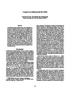
We have implemented a MAC version of QCSP-Solve (without CBJ). It performs AC, NI and the pure value rule as preprocessing and uses MAC, SDP and the pure value rule throughout search. We shall henceforth refer to QCSP-Solve with lexicographical value selection as LEX, and to QCSP-Solve with some heuristic as just the heuristic name. We initially used the same random problem generator as [3]. This generator creates three blocks of variables. The first block is existentially quantified, the second is universally quantified and the final block is again existentially quantified. Since ∃∀- and ∀∀-constraints could be removed by preprocessing, they are not generated. The generator has seven parameters: < n, n∀ , npos , d, p, q∀∃ , q∃∃ > where n is the total number of variables, n∀ is the number of universally quantified variables, npos is the position of the first universally quantified variable, d is the size of the domains, p is the fraction of constraints out of the possible ∀∃ and ∃∃ constraints, q∃∃ is the number of goods in ∃∃ constraints as a fraction of all possible tuples and q∀∃ is a similar quantity for ∀∃ constraints. A random total bijection from D(xi ) to D(xj ) is generated. (1 - q∀∃ ) is the fraction of tuples in the bijection which are conflicts, and all other tuples (both those in the bijection and those not) are goods. This method of generating ∀∃-constraints is used to allow generation of more random QCSPs which lack a flaw described in [27]. This flaw is when some combination of values assigned to some of the universal variables results in a domain wipe out of a future existential variable regardless of what values earlier existential variables are assigned. We generated 5000 test cases for each value of q∃∃ as shown in Figs. 1 and 2, comparing the mean average

run times and the number of nodes explored during search respectively, with a timeout of 1,000,000ms. Since we prevent the flaw described in [27], 98.9% of the problems generated have solutions, with all problems at q∃∃ ≥ 75 having a solution. We omit some of the heuristics from the figures for clarity: those omitted fall somewhere between DGP and LEX for q∃∃ = 50 to 80, and are higher than LEX for q∃∃ = 85 to 95. The graph is plotted with a log scale on the vertical axis. Adversarial Heuristics on 3-Block Problems SAS DSS SD LEX DGP

Avg Search Time (ms)

1000

100

50

55

60

65

70 Qee

75

80

85

90

Fig. 1. n = 21, n∀ = 7, d = 8, p = 0.20, q∀∃ = 1/2

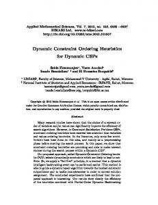
For q∃∃ = 50 to 80 we see that DGP, SAS and SD are faster than LEX, with the Dynamic Geelen’s Promise heuristic being consistently the fastest, with an improvement over LEX of up to 50%. Surprisingly, the dynamic heuristic, DSS, is slower than the static ones. In fact, as Figure 2 shows, DSS is slightly better than LEX in the number of search nodes it generates, but the overhead of calculating the support makes its runtime slower. However, for q∃∃ ≥ 85, all of the heuristics are slower than LEX. Investigating further, we can see that many of the heuristics also had slightly higher nodes than LEX, so it was not merely the calculation overheads causing them to be slower. In this region of the problem space, the heuristics appear to be making bad decisions. We used 5000 tests cases since on smaller test suites we observed a low chance (below 0.4%) of a generated problem in the q∃∃ = 60 to 70 range causing one or more heuristics to timeout and using those smaller suites would unfairly bias the results against those heuristics. These outliers each affected a different subset of the heuristics with no discernable pattern. The larger test suite obviously

Adversarial Heuristics on 3-Block Problems 1e+006

Avg Search Nodes Explored

SAS DSS SD LEX DGP

100000

10000

1000 50

55

60

65

70 Qee

75

80

85

90

Fig. 2. n = 21, n∀ = 7, d = 8, p = 0.20, q∀∃ = 1/2

included more outliers, but now they were spread more uniformly across the heuristics and q∃∃ points. However, none of the outliers adversely affected the performance of SAS, while LEX timed out on all of them. Even when we remove the outliers from the results, the heuristics still perform better than LEX on q∃∃ = 60 to 70, which is then the hardest region. In order to get a deeper insight into how the heuristics perform, we altered the problem generator to allow us to generate problems with an arbitrary number of blocks of variables. The parameters d, p, q∀∃ and q∃∃ all function the same in this new generator as the old, but a new parameter b is added for the size of the blocks. We ran the heuristics on 500 test cases of problems with 24 blocks, all of size 1 (i.e. where we have interleaved universal and existential quantifiers). We used 24 variables instead of 21 on these interleaved problems in order to get sufficiently difficult problems, as our initial tests on interleaved 21 variable problems ran too quickly for us to accurately distinguish between heuristics. For both problem types, if we fix 20% of the maximum amount of ∀∃-constraints and ∃∃-constraints, the amount of constraints out of the total possible constraints, when the preprocessable types are included, is different. For the 21 variable three-block problems we tested, there are 49 possible ∀∃-constraints, 91 possible ∃∃-constraints, 49 possible ∃∀-constraints and 21 possible ∀∀-constraints. So at p = 0.20 we generated 28 constraints out of 210 constraints, or 13.33% constraint density. For the 21 variable interleaved problems, there are 55 possible ∀∃-constraints, 55 possible ∃∃-constraints, 55 possible ∃∀-constraints and 45 possible ∀∀-constraints. So at p = 0.20 we generate 22 constraints out of 210

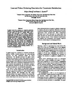
constraints, or 10.48% constraint density. The interleaved problems we generated are thus much sparser then three-block problems. It is also worth noting that these interleaved problems do not suffer heavily from the flaw described in [27]; in our randomly generated test cases, by q∃∃ = 40, 50% of the generated problems have solutions. For value of q∃∃ above 75, all problems had solutions. This means that none of these latter problems were flawed, so there is empirically less than a 0.2% chance of a flaw existing. Figure 3 shows the search time results of running the heuristics on these new problems (again, some heuristics are omitted for clarity). This time, the result was surprising. All of the heuristics, with the exception of Dynamic Average Support (DAS) and Dynamic Geelen’s Promise (DGP), are now worse than LEX for almost all values of q∃∃ . Figure 4 confirms that again these heuristics are also exploring more nodes than LEX. Adversarial Heuristics on Interleaved Problems

Avg Search Time (ms)

1000

100

SAS DAS SD LEX DGP 30

40

50

60 Qee

70

80

90

Fig. 3. n = 24, b = 1, d = 8, p = 0.20, q∀∃ = 1/2

Why should these heuristics perform so poorly on the interleaved problems? As a check, we implemented anti-heuristics, which reversed the value orderings, minimizing the chance of leading to a solution on existentially quantified variables and maximizing on the universally quantified variables. Figures 5 and 6 show a comparison between the SD heuristic and its anti-heuristic. On the three block problems, we can see the anti-heuristic performs worse than SD on the harder regions, but on the easier regions (e.g. q∃∃ ≥ 85) and on the interleaved problems the anti-heuristic performs better than SD does. Similar behaviour was visible for anti-heuristics of the other adversarial heuristics.

Adversarial Heuristics on Interleaved Problems

Avg Search Nodes Explored

1e+006

100000

10000

SAS DAS SD LEX DGP 1000 30

40

50

60 Qee

70

80

90

Fig. 4. n = 24, b = 1, d = 8, p = 0.20, q∀∃ = 1/2 Anti-heuristic on 3-Block Problems SD anti-SD

Avg Search Time (ms)

1000

100

50

55

60

65

70 Qee

75

80

Fig. 5. n = 21, n∀ = 7, d = 8, p = 0.20, q∀∃ = 1/2

85

90

Anti-heuristic on Interleaved Problems

Avg Search Time (ms)

1000

100

SD anti-SD 30

40

50

60 Qee

70

80

90

Fig. 6. n = 24, b = 1, d = 8, p = 0.20, q∀∃ = 1/2

To isolate the cause of these unexpected results, we first tried to identify the difference between the three block problems and the interleaved problems which might be the source of the change. We first checked to see if it was the lower density of the interleaved problems (as explained previously) which may be the source of the change in performance. However as Fig. 7 shows, on a three-block problem with 24 variables and approximately the same density as the interleaved tests, we do not see the same poor performance across all values of q∃∃ . For q∃∃ ≥ 75, though, all of the heuristics are slower than LEX. This is lower than on the p = 0.20 problems, so it appears that while density may influence the change, it is not the sole source of it. The issue appears to be a combination of sparse constraint graphs with loose constraints (high q∃∃ ). The interleaved problems have a higher ratio of ∀∃-constraints to ∃∃-constraints than the three-block problems. Owing to the nature of q∀∃ , these ∀∃-constraints are extremely loose. Therefore, the interleaved problems are both sparser and looser than the three-block problems. For sparse, loose problems, we can expect many value choices to lead to a solution, and it seems that optimising our measures is then counterproductive, and actually leads to more search. The reason why QCSPs are typically harder to solve than CSPs is the presence of the universally quantified variables. During the search, for a universal variable, to prove a solution we have to extend search trees down to the leaf nodes for every value in the domain. If adversarial heuristics are effectively favouring large universal domains in cases where many choices lead to a solution, then they would be increasing the size of the search space instead of reducing it. In

Lower Density 3-Block Problems DAS SSS SAS LEX

Avg Search Time (ms)

1000

100

30

40

50

60

70

80

90

Qee

Fig. 7. n = 24, n∀ = 8, d = 8, p = 0.14, q∀∃ = 1/2

QCSP-Solve, the main way of affecting the size of the universal domains is the Pure Value Rule, which identifies values in universal domains that are supported by all values in future domains, and removes them. On an existentially quantified variable, the adversarial heuristics attempt to maximize the support or domain size. The lexicographic ordering, however, is effectively random, and so on average it picks a value which results in smaller domains for the future variables than the other heuristics. If many choices lead to a solution (as in sparse loose problems), then the smaller domains are more likely to trigger the Pure Value Rule, reducing the size of the universal domains but still allowing a path to a solution, and hence less search for the solver. Similarly, the anti-heuristics minimise the domain size, and may benefit from this in sparse loose problems. The Pure Value Rule could also explain why the static heuristics performed better than the dynamic ones for 3-block problems. The dynamic heuristics make more informed choices, which produce on average larger future domains than the static heuristics. If we assume that even on most of the difficult problems the selections given by the static heuristics were good and extendable to solutions, then on average they would have smaller search trees.

5

Verification-focused Pure Value Heuristics

In the previous analysis, we saw that the work required to prove or disprove that a partial assignment leads to a solution may be significant, and we postulated that optimising measures that estimate the likelihood of a solution may sometimes lead to choices which increase the overall verification effort. We now

consider an alternative approach to value-ordering heuristics, where we try to choose values which require less effort for verification, regardless of whether or not they lead to a solution. This verification effort will depend on the features of the chosen solver, and thus it is likely that the heuristics will need to be tailored specifically for each solver. As before, we examine the behaviour of QCSP-Solve. Since the domain size of the universal domains has the most impact on search tree size, and QCSP-Solve’s pure value rule removes values from these domains, we develop heuristics which choose values which trigger the pure-value rule1 . We expect these heuristics to be most effective on sparse loose problems, where there are likely to be more solutions. The first heuristics are based on full application of the pure value rule. During search, we test each value by applying the Pure Value Rule to all future universal variables and count the number of values which would be pruned. We then generate three heuristics based on this count: Highest Average Pruning Full Pure Value (HAFPV) computes the average number of values pruned for future universal variables and selects values that maximise this, Lowest Smallest Domain Full Pure Value (LSFPV) computes the sizes of the future domains after pruning and chooses the value which results in the lowest smallest domain (tiebreaking to 2nd smallest, etc.) and finally Lowest Domain Product Full Pure Value (LPFPV) which computes the sizes of the future domains and chooses the value which has the lowest product of those domain sizes. The overhead of these heuristics is very large: approximately 80% of total runtime is spent generating the value ordering due to all the additional pure value calculations which are required. In comparison, for the adversarial domain heuristics less than 10% of runtime is spent on value ordering, and for the adversarial support heuristics it is generally less than 1%. To reduce the computational overhead, instead of directly calculating the pure values we can merely estimate how many pure values will be pruned. Again we have three variations on the basic heuristic: Highest Average Pruning Dynamic Pure Value Estimate (HADPVE),Lowest Smallest Domain Dynamic Pure Value Estimate (LSDPVE) and Lowest Domain Product Dynamic Pure Value Estimate (LPDPVE). Before search, the HADPVE heuristic preprocesses all existentially quantified variables after the first universally quantified variable. Every value a ∈ D(xi ), where xi is existentially quantified, is given a counter, P V estimatea, which starts at zero. Then a is checked against all values in the domains of the universally quantified variables before xi , and it is recorded whether the values support each other or not. If the values do not support each other, P V estimatea is incremented. Thus the counters P V estimatea become a counter for the maximum possible number of pure values which could be created by removing a from D(xi ). During search, HADPVE propagates after every value like the domain size heuristics, and then sums the P V estimates of all the values remaining in the domains of future existentially quantified variables. These 1

These heuristics can be viewed as analogous to the Block-Solve heuristic, which, although operating bottom-up, tries to minimise the branching effect of the universals to reduce search time.

sums are then ranked in ascending order, as the value with the lowest total is most likely to have created the most pure values. LSDPVE and LPDPVE perform similarly to HADPVE, except they have multiple P V estimates per value in each existential variable’s domain, which keep track of the estimated PV removals possible for the individual universal variables rather than just the total. LSDPVE and LPDPVE use these values to attempt to estimate the sizes of the future universal domains after the estimated pure values are removed. They then use these estimated universal domain sizes in the same way as their FPV counterparts.

Pure Value Heuristics on 3-Block Problems DGP LPFPV LSFPV HADPVE LSDPVE LEX

Avg Search Time (ms)

1000

100

10

50

55

60

65

70 Qee

75

80

85

90

Fig. 8. n = 21, n∀ = 7, d = 8, p = 0.20, q∀∃ = 1/2

We tested these new heuristics on the same problems as before, including DGP and LEX for comparison and excluding some of the pure value heuristics for clarity in the graphs. Figs. 8 and 9 show the results on the 3-block problems for search times and nodes explored, while Figs. 10 and 11 show the interleaved problem results. The first thing to note is that the FPV heuristics, despite their immense computational overhead, give significant run-time improvements over LEX when the value of q∃∃ is high. For other values of q∃∃ the FPV reduces the number of nodes explored, but the large overhead outweighs the benefit. HAFPV (omitted from the figures for clarity) and LPFPV both perform very similarly on all test cases, with LPFPV being slightly better for most values

Pure Value Heuristics on 3-Block Problems 1e+006 DGP LPFPV LSFPV HADPVE LSDPVE LEX Avg Search Nodes Explored

100000

10000

1000

100 50

55

60

65

70 Qee

75

80

85

90

Fig. 9. n = 21, n∀ = 7, d = 8, p = 0.20, q∀∃ = 1/2

of q∃∃ . LSFPV by its nature gives fewer pure value removals than HAFPV and LPFPV, so it is more effective on the more difficult 3-block problems which have fewer possible solutions and less effective on the other easier 3-block problems and the interleaved problems. LSDPVE and LPDPVE both performed significantly worse than HADPVE, due to the high inaccuracy of their estimations of the domain sizes after pruning. Since QCSP-Solve only calls the pure value rule on the current variable, there can be many values in the domains of future universals which are already prunable but have not yet been removed. Thus the true size of the universal domains is masked from LSDPVE and LPDPVE and so their attempts to choose the lowest minimum domain size will be inaccurate. Also the P Vestimates proved too inaccurate when used to count individual universal domains’ prunings as opposed to a measure of overall total prunings. Of these two heuristics, on 3Block problems LSDPVE was generally better, while on Interleaved problems LPDPVE was better. HADPVE, however, performs notably better. In the 3-block problems, it is the best heuristic on the tighter problems, and outperforms LEX on the loosest problems (although it is poorer in the middle of the range). On the interleaved problems, HADPVE outperforms LEX across the range, giving a speed-up of approximately 50% for almost all values of q∃∃ . It is only overtaken by the full

Pure Value Heuristics on Interleaved Problems

Avg Search Time (ms)

1000

100 DGP LPFPV LSFPV HADPVE LPDPVE LEX 30

40

50

60 Qee

70

80

90

Fig. 10. n = 24, b = 1, d = 8, p = 0.20, q∀∃ = 1/2 Pure Value Heuristics on Interleaved Problems 1e+006

Avg Search Nodes Explored

100000

10000

1000 DGP LPFPV LSFPV HADPVE LPDPVE LEX 100 30

40

50

60 Qee

70

Fig. 11. n = 24, b = 1, d = 8, p = 0.20, q∀∃ = 1/2

80

90

pure value heuristics at the higher values of q∃∃ . Note LPFPV is an order of magnitude better on nodes expanded than LEX on the interleaved problems.

6

Higher Density Problems

Finally, we consider the performance of the best of our heuristics on higher density problems. If our conjectures about sparse loose problems, the pure value rule and the universal domains are correct, then as we move to denser problems we should see the adversarial heuristics outperform the others. Figures 12 and 13 show our heuristics applied to three-block problems with a higher constraint density (40%). The performance of the SAS and DGP heuristics are consistently better than LEX for all values of q∃∃ , with the most noticeable improvements again in the harder region, where we again achieve approximately 50% improvements over LEX. This is as we would expect, since when the constraint graph is dense, we would not expect most choices to lead to solutions even with loose constraints, and so the conflict with the Pure Value Rule does not come into effect. The HADPVE heuristic performs slightly better than we expected, having slightly lower running times than LEX before the hard region, but then having a slower running time on the more difficult problems. Again, this poorer performance was expected, since the heuristic is likely to make choices leading to smaller future domains which are not extensible to solutions due to the higher constraint density. The LPFPV heuristic proved best of the FPV heuristics, and proved slower than LEX for most values of q∃∃ (though it was again better on search nodes explored) only improving on it at the highest values of q∃∃ but still performing worse than the adversarial heuristics. Problems with even higher densities showed the same behaviour. For higher density interleaved problems, we initially found that a large number (approximately 60%) of the randomly generated test cases possessed the flaw described in [27]. As such we altered the problem generator to only allow adding a new ∀∃-constraint to an existential variable if there are currently less than (d − 1) ∀∃-constraints on it already. In this way all flaws are prevented as it is impossible for the universals to cause a domain wipe out of an existential variable on their own. In addition, we reduced the problem size to 22 variables as at higher densities 24 variables were taking too long for all heuristics and LEX to run. Figures 14 and 15 show the performance on these flawless higher density (70%) interleaved problems. The three adversarial heuristics outperform LEX across the range, giving over a 50% decrease in run-times. Surprisingly the pure value heuristics proved to be very effective choices for high density interleaved problems. HADPVE is still a very good heuristic across all of the q∃∃ values. LPFPV becomes the best heuristic starting at q∃∃ = 93, showing a 50% reduction in run-time, and approaching an order of magnitude reduction at higher values of q∃∃ despite its extremely high overhead. For the number of search nodes expanded (Fig. 15), again we see that LPFPV is consistently an order of magnitude better than LEX.

Higher Density 3-Block Problems

100000

Avg Search Time (ms)

10000

1000

100

SAS HADPVE LPFPV DGP LEX

10 50

55

60

65

70 Qee

75

80

85

90

Fig. 12. n = 21, n∀ = 7, d = 8, p = 0.40, q∀∃ = 1/2

7

Conclusions and Future Work

We have introduced two approaches for designing value ordering heuristics for backtracking search in Quantified Constraint Satisfaction Problems. The first is solution-focused, and is a general approach derived from the minimax algorithm for adversarial search: for existential variables, choose values that maximise the chance of leading to a solution, and for universal variables, choose values that minimise the chance of leading to a solution. The chances of finding a solution are estimated by counting the number of supporting values in the future domains. The second approach is verification-focused, and aims to reduce the search effort required to show whether or not a partial assignment leads to a solution. We implement this approach for one particular solver, QCSP-Solve, by minimising the size of the universal domains through targeting the QCSPSolve Pure Value Rule. The heuristics show a 50% improvement in runtime over a lexicographic ordering on different classes of problem: the pure value heuristics are best suited to sparse loose problems, while the adversarial heuristics are best suited to dense problems. Finally, on dense interleaved problems both types of heuristic are up to 50% faster than lexicographic ordering, with one of the pure value heuristics, LPFPV, approaching an order of magnitude improvement. In future work, we plan to investigate enhanced use of the pure-value rule in heuristics for QCSP-Solve, and to investigate other implementations of the

Higher Density 3-Block Problems 1e+007

Avg Search Nodes Explored

1e+006

100000

10000

1000

100

SAS HADPVE LPFPV DGP LEX

10 50

55

60

65

70 Qee

75

80

85

90

Fig. 13. n = 21, n∀ = 7, d = 8, p = 0.40, q∀∃ = 1/2 Higher Density Interleaved Problems

Avg Search Time (ms)

100000

10000

1000

SAS DAS HADPVE LPFPV DGP LEX

100

70

75

80

85 Qee

90

Fig. 14. n = 22, b = 1, d = 8, p = 0.70, q∀∃ = 1/2

95

100

Higher Density Interleaved Problems 1e+008

Avg Search Nodes Explored

1e+007

1e+006

100000

10000

SAS DAS HADPVE LPFPV DGP LEX

1000

100 70

75

80

85 Qee

90

95

100

Fig. 15. n = 22, b = 1, d = 8, p = 0.70, q∀∃ = 1/2

verification-focused approach for other solvers, which will depend on how they handle the universal variables. Our work has shown that the ideal QCSP heuristic should do two things: it should make choices which will lead to a solution and it should make choices which minimise the search effort needed to show whether a partial assignment leads to a solution. The current two approaches each focus on only one of these aspects. The solution-focused approach seeks to make choices which lead to a solution, but may favour choices which require significant search effort to verify them. The verification-focused approach tries to reduce the search effort required to verify a partial assignment, but may do so by concentrating on existential choices which cannot be extended to a solution, and thus requiring more search. As future work, we will look for a hybrid heuristic which combines both approaches, making choices which lead to solutions, but favouring solutions which require less verification effort. The graphs of the nodes explored by the Full Pure Value heuristics show that there is a huge potential on many of the problem types for improving the search space reduction we can achieve, through the use of more intelligent value selection.

8

Acknowledgements

We wish to thank IRCSET and Microsoft for their financial support, Youssef Hamadi and Lucas Bordeaux for their comments, and the anonymous referees for their constructive suggestions.

References 1. Bordeaux, L., Monfroy, E.: Beyond NP: Arc-consistency for quantified constraints. In: Proceedings of CP. (2002) 371–386 2. Mamoulis, N., Stergiou, K.: Algorithms for quantified constraint satisfaction problems. In: Proceedings of CP. (2004) 752–756 3. Gent, I.P., Nightingale, P., Stergiou, K.: QCSP-Solve: A solver for quantified constraint satisfaction problems. In: Proceedings of IJCAI. (2005) 138–143 4. Geelen, P.A.: Dual viewpoint heuristics for binary constraint satisfaction problems. In: Proceedings of ECAI. (1992) 31–35 5. Frost, D., Dechter, R.: Look-ahead value ordering for constraint satisfaction problems. In: Proceedings of IJCAI. (1995) 572–578 6. Shannon, C.E.: Programming a computer for playing chess. Philosophical Magazine (Series 7) 41 (1950) 256–275 7. Haralick, R.M., Elliott, G.L.: Increasing tree search efficiency for constraint satisfaction problems. Artificial Intelligence 14(3) (1980) 263–313 8. Boerner, F., Bulatov, A., Jeavons, P., Krohkin, A.: Quantified constraints: Algorithms and complexity. In: Proceedings of CSL. (2003) 244–258 9. Bessiere, C., Verger, G.: Blocksolve: A bottom-up approach for solving quantified CSPs. In: Proceedings of CP. (2006) 635–649 10. Benedetti, M., Lallouet, A., Vautard, J.: Reusing CSP propagators for QCSPs. In: Proceedings of Workshop on Constraint Solving and Contraint Logic Programming, CSCLP. (2006) 63–77 11. Benedetti, M., Lallouet, A., Vautard, J.: QCSP made Practical by Virtue of Restricted Quantification. In: Proceedings of IJCAI. (2007) 38–43 12. Bessiere, C., Verger, G.: Strategic constraint satisfaction problems. In: Proceedings of CP Workshop on Modelling and Reformulation. (2006) 17–29 13. Ferguson, A., O’Sullivan, B.: Quantified Constraint Satisfaction: From Relaxations to Explanations. In: Proceedings of IJCAI. (2007) 74–79 14. Nightingale, P.: Consistency and the Quantified Constraint Satisfaction Problem. PhD thesis (2007) 15. Sabin, D., Freuder, E.C.: Contradicting conventional wisdom in constraint satisfaction. In: Proceedings of Second International Workshop on Principles and Practice of Constraint Programming (PPCP). Volume 874. (1994) 10–20 16. Prosser, P.: Hybrid algorithms for the constraint satisfaction problem. Computational Intelligence 9 (1993) 268–299 17. Freuder, E.C.: Eliminating interchangeable values in constraint satisfaction problems. In: Proceedings of AAAI. (1991) 227–233 18. Giunchiglia, E., Narizzano, M., Tacchella, A.: Backjumping for quantified boolean logic satisfiability. In: Proceedings of IJCAI. (2001) 275–281 19. Cadoli, M., Schaerf, M., Giovanardi, A., Giovanardi, M.: An algorithm to evaluate quantified boolean formulae and its experimental evaluation. Journal of Automated Reasoning 28(2) (2002) 101–142 20. Hulubei, T., O’Sullivan, B.: The impact of search heuristics on heavy-tailed behavior. Constraints Journal 11(2-3) (2006) 159–178 21. Bessiere, C., Regin, J.C.: MAC and combined heuristics: Two reasons to forsake FC (and CBJ?) on hard problems. In: Proceedings of CP. (1996) 61–75 22. Boussemart, F., Hemery, F., Lecoutre, C., Sais, L.: Boosting systematic search by weighting constraints. In: Proceedings of ECAI. (2004) 146–150

23. Refalo, P.: Impact-based search strategies for constraint programming. In: Proceedings of CP. (2004) 557–571 24. Cambazard, H., Jussien, N.: Identifying and exploiting problem structures using explanation-based constraint programming. Constraints 11(4) (2006) 295–313 25. Beck, J.C.;Prosser, P.R.: Variable ordering heuristics show promise. In: Proceedings of CP, LNCS, Springer (2004) 711–715 LNCS 3258. 26. Brown, K.N., Little, J., Creed, P.J., Freuder, E.C.: Adversarial constraint satisfaction by game-tree search. In: Proceedings of ECAI. (2004) 151–155 27. Gent, I.P., Nightingale, P., Rowley, A.: Encoding quantified CSPs as quantified boolean formulae. In: Proceedings of ECAI. (2004) 176–180