Journal of Diabetes Science and Technology
ORIGINAL ARTICLE
Volume 6, Issue 3, May 2012 © Diabetes Technology Society
Predicting Subcutaneous Glucose Concentration Using a LatentVariable-Based Statistical Method for Type 1 Diabetes Mellitus Chunhui Zhao, Ph.D.,1 Eyal Dassau, Ph.D.,1 Lois Jovanovič, M.D.,2 Howard C. Zisser, M.D.,2 Francis J. Doyle III, Ph.D.,1 and Dale E. Seborg, Ph.D.1
Abstract Background:
Accurate prediction of future glucose concentration for type 1 diabetes mellitus (T1DM) is needed to improve glycemic control and to facilitate proactive management before glucose concentrations reach undesirable concentrations. The availability of frequent glucose measurements, insulin infusion rates, and meal carbohydrate estimates can be used to good advantage to capture important information concerning glucose dynamics.
Methods:
This article evaluates the feasibility of using a latent variable (LV)-based statistical method to model glucose dynamics and to forecast future glucose concentrations for T1DM applications. The prediction models are developed using a proposed LV-based approach and are evaluated for retrospective clinical data from seven individuals with T1DM and for In silico simulations using the Food and Drug Administration-accepted University of Virginia/University of Padova metabolic simulator. This article provides comparisons of the prediction accuracy of the LV-based method with that of a standard modeling alternative. The influence of key design parameters on the performance of the LV-based method is also illustrated.
Results:
In general, the LV-based method provided improved prediction accuracy in comparison with conventional autoregressive (AR) models and autoregressive with exogenous input (ARX) models. For larger prediction horizons (≥30 min), the LV-based model with exogenous inputs achieved the best prediction performance based on a paired t-test (α = 0.05).
Conclusions:
The LV-based method resulted in models whose glucose prediction accuracy was as least as good as the accuracies of standard AR/ARX models and a simple model-free approach. Furthermore, the new approach is less sensitive to changing conditions and the effect of key design parameters. J Diabetes Sci Technol 2012;6(3):617-633
Author Affiliations: 1Department of Chemical Engineering, University of California, Santa Barbara, Santa Barbara, California; and 2Sansum Diabetes Research Institute, Santa Barbara, California Abbreviations: (AR) autoregressive, (ARX) autoregressive with exogenous input, (CCA) canonical correlation analysis, (CG) continuous glucose, (CGM) continuous glucose monitoring, (CHO) carbohydrate, (CVP) constant value prediction, (EGA) error-grid analysis, (FDA) Food and Drug Administration, (I:C) insulin-to-carbohydrate ratio, (LV) latent variable, (LVX) latent variable with exogenous input, (MAD) mean absolute deviation, (PLS) partial least squares, (RMSE) root mean-square error, (T1DM) type 1 diabetes mellitus, (UVa/Padova) University of Virginia/ University of Padova Keywords: autoregressive model, autoregressive model with exogenous inputs, continuous glucose monitoring, glucose concentration prediction, latent variable model, latent variable model with exogenous inputs, type 1 diabetes mellitus Corresponding Author: Dale E. Seborg, Ph.D., Department of Chemical Engineering, University of California, Santa Barbara, Santa Barbara, CA 93106-5080; email address
[email protected] 617
Predicting Subcutaneous Glucose Concentration Using a LatentVariable-Based Statistical Method for Type 1 Diabetes Mellitus
Zhao
Introduction
T
ype 1 diabetes mellitus (T1DM) is a disease characterized by the inability of the body to regulate blood glucose concentration. Type 1 diabetes mellitus results from autoimmune destruction of pancreatic β cells, which produce the hormone insulin. Without appropriate treatment with exogenous insulin, people with T1DM have difficulty maintaining their blood glucose concentration within a normal range (e.g., 70–150 mg/dl). Consequently, they can suffer from large glycemic excursions, including episodes with very low glucose levels (hypoglycemia) and very high glucose levels (hyperglycemia); both situations are detrimental to the quality of life.1
Insulin boluses are commonly taken simultaneously with meals and in a specified ratio to the meal carbohydrates (CHOs).2 From a modeling perspective, insulin boluses and meal CHOs are two input variables that affect the output variable, blood glucose concentration. A careful balance is required between a person’s daily activities, diet, and insulin administration in order to sustain the blood glucose concentration in the near-normal range. This balancing is not an easy task, because large glycemic variations often go undetected, including asymptomatic hypoglycemia or hypoglycemia unawareness.2 Developments in continuous glucose monitoring (CGM) devices have created new opportunities for improved glycemia management of T1DM. For commercial CGM devices, frequent glucose measurements (e.g., every 1–5 min) are displayed in real time, which provide important information about a person’s current glycemic state and its trend. If the recent glucose history follows previous known patterns, future blood glucose values can be anticipated from past experience.3 In particular, an empirical model of glucose dynamics can facilitate glucose management. A model-based controller for an artificial pancreas has the potential to automatically regulate blood glucose levels based on available glucose measurements, insulin infusion and meal information, and model predictions of future glucose trends. Thus the identification of simple, accurate glucose prediction models is a key step in the development of an effective artificial pancreas. Many empirical (or “data-driven”) modeling techniques have been evaluated in both in silico and clinical studies.4–14
J Diabetes Sci Technol Vol 6, Issue 3, May 2012
618
The existing dynamic empirical models for T1DM include linear input–output models and nonlinear models such as neural networks, as summarized by Finan and colleagues.4 Bremer and Gough3 first suggested that glucose time-series data had an inherent structure that could be described by a simple linear dynamic model. The linear models that have received the most attention for T1DM applications are autoregressive (AR) models and autoregressive with exogenous inputs (ARX) models. Only CGM data are required to develop an AR model and to predict future glucose concentrations as a linear combination of recent measurements. Cobelli and associates5,6 have proposed low-order AR models and polynomial models with time-varying parameters determined by weighted least squares. Reifman and colleagues7 have clinically evaluated subject-specific AR models with high model orders in order to improve management of glucose concentrations. Eren-Oruklu and coworkers8,9 have reported subject-specific recursive AR models wherein the model parameters were recursively updated to reflect the recent glucose history. The ARX models are an extension of AR models to include two exogenous inputs: insulin delivery and meal CHOs. Finan and collaborators4,10,11 have developed ARX models for in silico and human subjects. They also analyzed the effect of design parameters such as input excitation on glucose prediction performance. Both AR and ARX model parameters can be easily estimated using standard least squares analysis. Other modeling techniques such as radial basis function, neural network models,13–15 and Kalman filters12,16,17 have also been reported. Multivariate statistical methods18,19 based on the fundamental concept of latent variables (LVs), such as partial least squares (PLS) and principal component analysis, have proven to be powerful tools for data analysis, modeling, and prediction. Although there have been many successful applications in the process industries, few applications20 have been reported for T1DM. In this paper, a LV-based technique21 is employed to develop an empirical glucose prediction model from T1DM subject data. The LV-based modeling technique consists of two steps. First, a PLS model is developed to predict future glucose concentrations (the model output)
www.journalofdst.org
Predicting Subcutaneous Glucose Concentration Using a LatentVariable-Based Statistical Method for Type 1 Diabetes Mellitus
Zhao
from available time series data for the predictor variables: glucose measurements, insulin boluses, and meal CHO estimates (the model inputs). The PLS model is based on a small number of uncorrelated LVs. In the second step, the PLS model is improved by postprocessing using canonical correlation analysis (CCA).21 In general, the T1DM data are highly correlated due to the small sampling period for glucose measurement and because the insulin bolus is calculated to be a constant ratio of the estimated meal CHOs. By contrast, LVs are a small number of uncorrelated variables that are linear combinations of the predictor variables. In this article the LV-based prediction method is evaluated using both retrospective clinical data and in silico prospective simulations. The clinical data for seven subjects were collected at the Sansum Diabetes Research Institute in Santa Barbara, CA. In silico evaluation was performed for 10 adult subjects who were simulated using the Food and Drug Administration (FDA)-accepted University of Virginia/University of Padova (UVa/Padova) metabolic simulator.22 This article provides comparisons of the prediction accuracy of the LV-based method with the accuracy of a standard modeling alternative, the ARX method. The performance of the LV-based method to the choice of key design parameters is also illustrated.
output variable. Thus the first LV (or score) t1 can be expressed as t1 = Xw1
where X(N × Jx) is the predictor data matrix wherein N is the number of samples and Jx is the number of predictor variables. The first weight vector w1 is a value of w that maximizes the objective function: arg max (w TXT yy TXw) w
subject to w T w = 1
(2)
where vector y(N × 1) denotes the output variable data. Thus w1 is the eigenvector that corresponds to the largest eigenvalue of matrix XT yy TX. The second weight w2 is calculated in a similar manner after X and y have been deflated by t1: p1T = (t1T t1) –1 t1TX
Methodology Latent-Variable-Based Statistical Analysis
The LV-based models for this paper are empirical, linear dynamic models that predict an output variable, future glucose concentration from past glucose measurements, insulin boluses, and meal CHO estimates (the predictor variables). Because these predictor data tend to be highly correlated, multivariable statistical methods are a natural choice since they have the ability to analyze large amounts of highly correlated data. The underlying assumption is that the predictor data can be described by a small number of orthogonal LVs that can be directly linked to the output variable via regression analysis.
A variety of LV-based regression methods have been developed, with the chief difference being how the LVs are calculated. A general comparison of LV-based methods has been reported by Burnham and associates.23 The LV-based methods used in this paper are briefly described here.
(3)
E1 = X – t1p1T
(4)
q1 = (t1T t1) –1 t1T y
(5)
f 1 = y – t 1q 1
(6)
where p1 and q1 are the PLS loadings for the predictor variables and the output variable, respectively. In order to calculate w2, the calculation in Equation (2) is repeated with E1 and f1 replacing X and y, respectively. The remaining weight vectors are also calculated using this iterative procedure. The number of LVs in the PLS model, NLV, is an important design parameter that can be as large as the rank of X. In this paper, an appropriate value of NLV was determined by cross validation. Next, the weight vectors w1, w2,… are collected in a weight matrix W while the loadings for the predictor variables and the output variable are collected in matrix P and vector q, respectively. Finally, the score vectors t1, t 2,… are arranged as the columns of matrix T. Then the output variable prediction is given by ŷ = XRq = Tq
(7)
R = W(PTW) –1
(8)
where
Partial least squares18,23–25 is a common LV-based regression method. The LVs are linear combinations of the predictor variables that result in maximal covariance with the
J Diabetes Sci Technol Vol 6, Issue 3, May 2012
(1)
619
www.journalofdst.org
Predicting Subcutaneous Glucose Concentration Using a LatentVariable-Based Statistical Method for Type 1 Diabetes Mellitus
Zhao
A classical PLS calculation procedure is described by Lindgren and colleagues.25 One problem associated with the PLS method requires special attention. The PLS objective is to model the variations in X and maximize their covariance with y, but large covariance does not necessarily mean strong correlation. When the predictor matrix X contains a considerable amount of process variations that are uncorrelated with y, it is possible that the PLS LVs may capture the major systematic variations in the predictors X but only have relatively weak correlation with y. This situation leads to a complex model structure and an overfitting problem. Unlike PLS, CCA26–28 inherently ignores the variations in X that are uncorrelated with y and directly maximizes the variations that are correlated with y. The CCA objective function is to determine the weight vectors w so that arg max (w TXT y) w
subject to w TXTXw = 1
(9)
The first weight vector w 1 is the eigenvector corresponding to the largest eigenvalue of matrix (XTX) –1 XT y(y T y) –1y TX. The maximum number of CCA LVs can be up to Lcca = min (Jx,Jy), where Jx and Jy are the numbers of predictor and output variables, respectively. In this paper, a single output variable is considered, thus Lcca = 1. A comparison of Equations (2) and (9) indicates that the CCA objective is to maximize correlation, while the PLS objective is to maximize covariance. For CCA, the single LV and loading for the output variable are calculated as t = Xw
(10)
q = (t T t) –1 t T y = t T y
(11)
Finally, the output prediction is given by ŷ = Xwq = Tq
(12)
Unfortunately, directly applying CCA to the {X, y} data can lead to ill-conditioned problems resulting from the (XTX) –1 term in the calculations. To avoid this problem, Yu and MacGregor21 have suggested a two-step LV-based modeling algorithm (PLS-CCA), where CCA is used as a postprocessing technique to further improve the PLS J Diabetes Sci Technol Vol 6, Issue 3, May 2012
620
LVs. In this way, a parsimonious regression model with the same prediction ability as the standard PLS model can be obtained. Based on these considerations, their PLS-CCA algorithm is employed in this paper to develop the empirical model for glucose concentration prediction. Compared with the conventional AR and ARX modeling methods, the y-related variability in the predictor data is modeled by only a few LVs, which are calculated in order based on their relationship with future glucose values.
Latent Variable/Latent Variable with Exogenous Input Prediction Model
In order to apply the LV-based modeling technique, the predictor and output data sets must be organized in an appropriate manner. For both the simulation and the clinical studies, the predictor data were available for multiple days using a 5 min sampling period. Previous publications from our research group10,11,29 have demonstrated that model accuracy improves when the exogenous input data are preprocessed prior to model identification. The preprocessing consists of passing each input impulse (i.e., the insulin boluses and CHO estimates) through a simple transfer function model, thus producing time-smoothed inputs. In this paper, the second-order transfer function models reported by Grosman and coworkers29 are used. The data arrangement procedure is described in Appendix A.
The training data {X, y} are normalized to zero mean and unit variance, respectively, which reduces the data nonlinearity to some extent. After applying the PLS-CCA approach to the normalized data, the final LV-based regression model can be readily calculated: t c = Xwc
(13)
qc = (t cT t c) –1 t cT y
(14)
ŷc = t c qc
(15)
where wc(Jx × 1) is the single PLS-CCA weight vector. Latent variable t c is a linear combination of the predictor variables and weight vector wc(Jx × 1), indicating the systematic variations in predictor variables that are closely related to the output variable. The vector of prediction errors f is defined f = y – ŷc
(16)
The two-step modeling method can be summarized as follows. First, the PLS LVs are calculated, and then CCA www.journalofdst.org
Predicting Subcutaneous Glucose Concentration Using a LatentVariable-Based Statistical Method for Type 1 Diabetes Mellitus
Zhao
is used to further process them and to calculate the final predictions in Equation (15). In this paper, only one PLS-CCA LV can be used because of the single output variable, regardless of the number of PLS LVs. Thus, only the underlying systematic glycemic variability that is closely related to the output variable (predicted glucose concentration) is captured by the single PLS-CCA LV. The loading coefficient for the output variable, scalar qc, is obtained by regressing y on t c, which indicates how much t c contributes to y. Then the future glucose prediction ŷc and the prediction error f(N × 1) can be calculated. A flowchart for the proposed modeling strategy is given in Figure 1. The key MATLAB m-files for model development are shown in Appendices B and C. The developed latent variable with exogenous input (LVX)/LV model is then used for online application to new data. During the online application, the newly available predictor vector xnewT(1 × Jx) at each sampling instant can be expressed as [gnewT(1 × LG), u I,newT(1 × LI), u M,newT(1 × L M)], where LG is the number of current and past glucose measurements and LI and L M are the corresponding values for the insulin boluses and meal CHO estimates, respectively. The data normalization of xnewT is based on information obtained from training data; then the normalized xnewT is projected onto the LVX/LV model in order to make the PH-step-ahead prediction, ŷnew. The prediction error fnew can be calculated after PH samples when the new measurement ynew becomes available: tnew = xnewT wc
(17)
ŷnew = tnew qc
(18)
fnew = ynew – ŷnew
(19)
For LV-based prediction models, the important design parameters are
Figure 1. A schematic representation of the modeling method (L*: for LVX modeling, it includes the values of L G, LI, and LM as well as the input time delay D I and D M, while for LV modeling, it only includes the value of L G). 1The detailed PLS-CCA modeling procedure is shown by MATLAB code in Appendix B. 2The detailed prediction procedure is shown by MATLAB code in Appendix C.
1. Δt, the data sampling period; 2. Jx, the predictor length, i.e., the number of samples in each row of predictor matrix X; 3. PH, the prediction horizon (expressed as the number of samples into the future); and
For clarity, the resulting LV-based glucose prediction model will be denoted as an LVX model when the exogenous inputs (bolus insulin and meal CHOs) are included in the predictor matrix X and as an LV model when they are not. For comparison, the conventional
4. NLV, the number of LVs that are used in the PLS model.
J Diabetes Sci Technol Vol 6, Issue 3, May 2012
621
www.journalofdst.org
Predicting Subcutaneous Glucose Concentration Using a LatentVariable-Based Statistical Method for Type 1 Diabetes Mellitus
Zhao
AR and ARX models are described in Appendix D. For online applications, the future input measurements for the LVX and ARX models are assumed to be zero. However, the smoothed future meal and insulin-related signals generated using data available at the current time are used for prediction.
Glucose predictor length LG was evaluated to assess its effects on prediction performance. On one hand, a larger LG value will increase the predictor information for the glucose prediction, which may improve prediction accuracy. On the other hand, if LG is too large, the oldest information may not be useful for prediction and thus actually reduce prediction accuracy.
Results and Discussion In Silico Study
The simulated subject data were generated for a 5 min sampling period using the FDA-accepted UVa/Padova metabolic simulator.22 The simulations included a threemeal scenario for breakfast, lunch, and dinner taken at approximately 7:00 am, 12:00 pm, and 6:00 pm with 40, 85, and 60 g of CHO, respectively. An optimal bolus insulin was given immediately based on the ideal insulin-tocarbohydrate ratio (I:C). This situation is used as the nominal case for model identification. Three additional cases were considered to assess the performance of the identified models to nonideal situations: Case I: The meal timing and CHO meal content were varied to represent variations in daily life. Thus a 1 h shift (forward or backward) in meal timing and ±75% variation in CHO amount were implemented. Case II: In addition to the meal variations of case I, a 30% increase in I:C was considered, which resulted in lower peak glucose measurements.
RMSE =
1 N
S(y – ŷ )
i∈N
i
i
2
(20)
where ŷi is the predicted value, yi is the CGM measurement, and N is the number of samples. The other metric is the continuous glucose (CG) errorgrid analysis (EGA),30,31 which is specific to diabetes applications. Here CGM data are used as the reference for analyzing how accurate the glucose predictions are according to the CG-EGA metric. In the following results, the EGA label refers to the percentage of the model predictions that lie in the “clinically accurate” region A. The optimal value of LG was either 7 or 8 for both the LV and the AR models and for all subjects. For the ARX and LVX models, the optimal numbers of LI and L M were more subject dependent, as were the input time delays, kins and kmeal, in Appendix D. An additional 5 days of simulated testing data were used to evaluate model accuracy.
Case III: It is the same as case I except that a 30% decrease in the I:C was considered, which resulted in higher peak glucose measurements. Cases II and III were used to test whether the identified prediction model for the nominal case is valid due to inaccurate CHO estimates. Training data for model identification consisted of 2 days of simulated data (midnight to midnight) for the nominal case. The impulse inputs were transformed by secondorder transfer functions29 into continuous impulse outputs. One day of training data was used for model identification, while the second day of training data was used for cross-validation to choose design parameters, PH, and the numbers of past measurements that were included in the predictor matrix. The latter are referred to as predictor lengths and denoted as LG, LI, and L M for glucose, insulin bolus, and meal CHO estimate, respectively. (See Appendix A.)
J Diabetes Sci Technol Vol 6, Issue 3, May 2012
The prediction accuracy of the identified models can be evaluated and compared using several standard metrics.4,8,10 In this paper, two metrics are used. One metric is the root mean-square error (RMSE), which is defined as
622
Figure 2 shows the influence of glucose predictor length LG on model accuracy for the four identification methods, three cases, and a prediction horizon of 30 min (i.e., PH = 6). The RMSE values in Figure 2 for cases I–III are averages for the 10 in silico subjects and five days of testing data. For case I, the RMSE index for all four models is insensitive to changes in LG for LG > 7. For nonideal cases II and III, the ARX model performance is rather erratic and becomes worse as LG increases. For a specific value of LG, the LVX model is the most accurate model based on the RMSE metric and a paired t-test for individual subjects (α = 0.05). These LV and AR models exhibit similar prediction accuracy, and their differences are not statistically significant based on a paired t-test (α = 0.05).
www.journalofdst.org
Predicting Subcutaneous Glucose Concentration Using a LatentVariable-Based Statistical Method for Type 1 Diabetes Mellitus
Zhao
The choice of prediction horizon PH involves a trade-off. It should be large enough to ensure adequate time for a necessary intervention or corrective action in order to avoid abnormal glycemia. On the other hand, a larger PH value may result in less accurate glucose predictions. Figure 3 shows the prediction accuracy for different identification methods and PH values up to 12 when the optimal values of LG were used for different methods and subjects. The RMSE values were averaged for 10 adults and five days of testing data. As expected, the prediction accuracy decreases as PH increases. For PH ≥ 6, the differences in prediction accuracy for the four types
Figure 2. Comparison of the average RMSE values for 10 in silico subjects and different models with respect to effects of glucose predictor length L G on 30 min glucose prediction. (A) case I, (B) case II, (C) case III.
J Diabetes Sci Technol Vol 6, Issue 3, May 2012
of models become more significant. The LVX model is statistically more accurate based on a paired t-test (α = 0.05) for cases II and III; for case I, its accuracy is similar to that of the ARX model. The LV and AR models achieve similar accuracy and the differences are not statistically significant based on a paired t-test (α = 0.05). Figures 2 and 3 demonstrate that an ARX model developed for the nominal case conditions is less accurate for cases II and III, in comparison with the other methods. The number of LVs for the PLS calculations, NLV, determines how much predictor information is retained in the PLS model. In general, using a small value of NLV indicates that much of the information in the predictor
Figure 3. The effect of prediction horizon PH on model prediction accuray for 10 in silico subjects and different modeling techniques. Average RMSE values for (A) case I, (B) case II, (C) case III.
623
www.journalofdst.org
Predicting Subcutaneous Glucose Concentration Using a LatentVariable-Based Statistical Method for Type 1 Diabetes Mellitus
Zhao
data X is considered to be uninformative for prediction purposes and thus is excluded from the PLS model. Preliminary simulations indicated that a value of NLV = 4 or 5 gave good results.
free method, constant value prediction (CVP). In this approach, the prediction PH samples ahead is simply the current value.
Figure 4 compares model accuracy for subject #1, 30 min predictions, cases I–III, and a representative day of testing data. For case I, both the ARX and LVX models capture the general glucose trend with similar accuracy. For cases II and III, the ARX model provides less accurate predictions at the peaks of the glucose profiles. Similar conclusions occur for subject #7 in Figure 5, where a representative day of test data is considered for the three cases. Tables 1 and 2 summarize model prediction accuracy for the 10 in silico adults based on two metrics, RMSE (mg/dl) and EGA (%) in region A. Both the mean absolute deviation (MAD) and median average deviation values are shown. The shaded values in a column indicate models that are statistically superior compared with the unshaded models in the column, based on a paired t-test (α = 0.05). Tables 1 and 2 also include results for a simple model-
Figure 4. Comparison of measured values and 30 min predictions for LVX and ARX models and in silico subject #1 over a one-day period: (A) case I, (B) case II, and (C) case III. A green left triangle indicates the time of a meal and an insulin bolus injection, which are taken at the same time.
J Diabetes Sci Technol Vol 6, Issue 3, May 2012
In general, the LVX model in Table 1 gives the lowest RMSE values and thus is the most accurate. For case I, all four modeling methods are superior to the CVP approach. But for cases II and III, the ARX model usually gives worse results than the CVP approach. For the EGA (%) results in Table 2, all models except ARX give better results for case III than for cases I and II, even though this trend is not present for the RMSE values in Table 1. This anomaly occurs because the glucose values are higher for case III due to insulin underdelivery. Region A of the EGA becomes larger when the glucose values are higher. From this viewpoint, the EGA index is a less sensitive metric than the RMSE index.
Figure 5. Comparison of measured values and 30 min predictions for LVX and ARX models and in silico subject #7 over a one-day period: (A) case I, (B) case II, and (C) case III. A green left triangle indicates the time of a meal and an insulin bolus injection, which are taken at the same time.
624
www.journalofdst.org
Predicting Subcutaneous Glucose Concentration Using a LatentVariable-Based Statistical Method for Type 1 Diabetes Mellitus
Zhao
Table 1. Root Mean-Square Error Results (mg/dl; Mean ± Mean Absolute Deviation) for Glucose Prediction and 10 in Silico Subjects PH = 6 (30 min)
PH = 12 (60 min)
Case I
Case II
Case III
Case I
Case II
Case III
LVX
8.9 ± 0.7
8.5 ± 0.6
8.4 ± 0.6
14.6 ± 1.2
13.5 ± 1.7
13.9 ± 1.9
ARX
9.8 ± 0.5
14.7 ± 3.7
13.6 ± 3.4
14.9 ± 1.1
27.7 ± 9.7
24.8 ± 8.8
LV
11.2 ± 1.1
11.5 ± 1.1
11.3 ± 1.2
18.8 ± 3.1
19.8 ± 2.9
19.1 ± 3.5
AR
11.6 ± 1.1
11.6 ± 1.2
11.6 ± 1.1
20.0 ± 2.6
20.0 ± 2.6
20.1 ± 2.5
CVP
13.9 ± 1.8
13.9 ± 1.8
13.9 ± 1.7
22.2 ± 3.2
22.3 ± 3.3
22.3 ± 3.1
Table 2. Error-Grid Analysis Results (% in Region A; Mean ± Mean Absolute Deviation) for Glucose Prediction and 10 in Silico Subjects PH = 6 (30 min) LVX
PH = 12 (60 min)
Case I
Case II
Case III
Case I
Case II
Case III
97.9 ± 0.7
95.2 ± 0.5
99.1 ± 0.8
89.7 ± 2.3
78.8 ± 4.1
92.8 ± 3.7
ARX
97.8 ± 0.8
91.1 ± 3.2
96.9 ± 2.4
89.7 ± 2.6
74.0 ± 4.2
88.7 ± 6.5
LV
96.4 ± 1.5
93.5 ± 1.4
98.2 ± 1.0
83.5 ± 5.3
76.1 ± 4.9
89.9 ± 4.2
AR
97.1 ± 1.0
94.9 ± 1.0
98.6 ± 0.6
83.7 ± 3.6
78.2 ± 3.9
89.6 ± 2.4
CVP
94.3 ± 1.9
90.6 ± 2.2
97.0 ± 1.3
82.0 ± 4.5
76.2 ± 4.3
87.4 ± 3.9
Retrospective Clinical Data
The two impulse inputs were transformed into timesmoothed inputs using the second-order transfer functions of a previous study.29 The estimated model predictor lengths and input time delays were selected based on cross validation. The optimal predictor length LG for glucose was 7 or 8 for all empirical models and subjects. For ARX and LVX models, the optimal model parameters for two exogenous inputs are more subject dependent, including the predictor lengths and input time delays. The identified prediction models were then tested using other segments of data for each subject.
In the retrospective clinical evaluation, several days of data for each of the seven ambulatory subjects were available. The subjects had given their voluntary and written informed consent to participate in the study. The key characteristics for the seven subjects (four males and three females) are • Age: 48 ± 15 years • Weight: 87 ± 25 kg
The weak influence of LG on model accuracy is illustrated in Figure 6 for 30 min predictions and test data. The mean RMSE value and MAD from median value are shown for the seven clinical subjects. Based on a paired t-test (α = 0.05) for individual subjects, the LVX model is statistically superior to the other models.
• Height: 174 ± 11 cm • Correction factor: 35 ± 14 mg/dl/U • I:C: 1:9 ± 1:2 U/g The CGM glucose data were collected using a DexCom 7 PlusTM device (DexCom, San Diego) with a 5 min sampling period. The estimated meal CHO values and recorded insulin boluses were used as the exogenous inputs. The data were divided into 24 h time segments from 4:00 am to 4:00 am. One day of data was used for model identification.
J Diabetes Sci Technol Vol 6, Issue 3, May 2012
The effect of prediction horizon PH on average prediction performance is shown in Figure 7. The optimal predictor length LG for glucose was used for different empirical models and subjects. As expected, as PH increases, the average RMSE value increases and the MAD of the RMSE index also increases. The four types of models produce
625
www.journalofdst.org
Predicting Subcutaneous Glucose Concentration Using a LatentVariable-Based Statistical Method for Type 1 Diabetes Mellitus
Zhao
Figure 7. The effect of prediction horizon PH on model prediction accuracy for seven clinical subjects and different modeling techniques. (A) mean RMSE (mg/dl); (B) MAD of RMSE (mg/dl). Figure 6. The effect of glucose predictor length L G on model prediction accuracy for seven clinical subjects, PH = 6, and different modeling techniques. (A) mean RMSE (mg/dl); (B) MAD of RMSE (mg/dl).
Table 3. Root Mean-Square Error Results (mg/dl; Mean ± Mean Absolute Deviation) for Glucose Prediction and Seven Clinical Subjects
essentially the same prediction accuracy for small values of PH. However, when PH ≥ 6, the LVX model is the most accurate, while the AR model is the least accurate. For PH ≥ 6, a paired t-test (α = 0.05) indicates that the LVX model is usually statistically superior to the other methods.
Methods
The measured and predicted glucose profiles for the LVX and ARX models are shown in Figure 8 for two representative subjects and one day of test data. The ARX and LVX models give similar results for the two subjects. Similar results are shown in Figure 9 for AR and LV models for the same two subjects.
PH = 6 (30 min)
PH = 9 (45 min)
PH = 12 (60 min)
LVX
11.1 ± 2.4
18.7 ± 3.7
24.4 ± 4.7
29.2 ± 5.5
ARX
11.3 ± 2.5
19.5 ± 3.8
25.5 ± 4.6
30.3 ± 5.3
LV
11.3 ± 2.4
19.7 ± 3.3
26.0 ± 3.8
31.2 ± 4.0
AR
11.6 ± 2.4
20.8 ± 3.5
28.3 ± 4.2
34.9 ± 4.5
CVP
21.7 ± 3.8
26.9 ± 3.2
31.0 ± 2.9
37.5 ± 2.5
Table 4. Error-Grid Analysis Results (% in Region A; Mean ± Mean Absolute Deviation) for Glucose Prediction and Seven Clinical Subjects
Tables 3 and 4 summarize model prediction accuracy for the seven clinical subjects based on RMSE (mg/dl) and EGA (% in region A), respectively. The shaded values in a column indicate models that are statistically superior compared with the unshaded models in the column, based on a paired t-test (α = 0.05). All four modeling techniques were much more accurate than the CVP model-free method. For PH = 3, the four modeling
J Diabetes Sci Technol Vol 6, Issue 3, May 2012
PH = 3 (15 min)
626
Methods
PH = 3 (15 min)
PH = 6 (30 min)
PH = 9 (45 min)
PH = 12 (60 min)
LVX
96.8 ± 1.8
86.1 ± 7.5
78.8 ± 9.9
72.1 ± 10.6
ARX
96.5 ± 2.1
84.9 ± 7.9
77.5 ± 8.8
70.1 ± 10.3
LV
96.4 ± 2.0
84.9 ± 7.6
76.3 ± 10.2
68.4 ± 9.6
AR
96.2 ± 2.3
84.4 ± 7.5
74.8 ± 8.8
66.5 ± 9.8
CVP
84.0 ± 5.8
76.9 ± 6.1
71.1 ± 6.6
63.0 ± 6.2
www.journalofdst.org
Predicting Subcutaneous Glucose Concentration Using a LatentVariable-Based Statistical Method for Type 1 Diabetes Mellitus
Zhao
Figure 8. Comparison of glucose data and 30 min predictions for the LVX and ARX models and one day of test data. (A) subject #1; (B) subject #5. A green left triangle indicates the time of a meal and a red right triangle indicates the time of an insulin bolus.
Figure 9. Comparison of glucose data and 30 min predictions for the LV and AR models and one day of test data. (A) subject #1; (B) subject #5. A green left triangle indicates the time of a meal and a red right triangle indicates the time of an insulin bolus.
methods exhibit similar prediction performance. But as PH increases, the differences become significant. For PH ≥ 6, the LVX models in Table 3 are statistically superior, as indicated by a paired t-test (α = 0.05) for the RMSE index.
For retrospective clinical data, the LV and LVX models provided modest improvements in prediction accuracy compared with the corresponding standard models (AR and ARX). For PH ≥ 6, the inclusion of exogenous inputs in the models (LVX and ARX) resulted in more accurate models compared with the models without exogenous inputs (LV and AR), respectively.
Conclusions Glucose prediction models based on a LV-based approach have been evaluated for both an in silico study and a retrospective analysis of clinical data. The new LV and LVX models were compared with standard AR and ARX models and a simple model-free approach (CVP), where the future prediction is merely set equal to the current value. For both investigations, the empirical models were more accurate than the model-free method.
These promising modeling results should encourage extensions of this research methodology. For example, a critical problem concerns the generation of hypoglycemic event alerts based on an online statistical analysis of current and past data.
For the in silico study, the LV-based modeling method gave more accurate predictions than the AR/ARX alternative for changing conditions such as meal timing, meal amounts, and I:C. For large prediction horizons (≥30 min), the LVX model was statistically superior to LV and AR models based on a paired t-test (α = 0.05) for all cases and superior to the ARX models for cases II and III. J Diabetes Sci Technol Vol 6, Issue 3, May 2012
627
Funding: The research work was supported by the Juvenile Diabetes Research Foundation (grants 22-2009-797, 22-2009-76) and the National Institutes of Health (DK085628-01).
www.journalofdst.org
Predicting Subcutaneous Glucose Concentration Using a LatentVariable-Based Statistical Method for Type 1 Diabetes Mellitus
Zhao
References: 1. Rubin RR, Peyrot M. Quality of life and diabetes. Diabetes Metab Res Rev. 1999;15(3):205–18. 2. Rabasa-Lhoret R, Garon J, Langelier H, Poisson D, Chiasson JL. Effects of meal carbohydrate content on insulin requirements in type 1 diabetic patients treated intensively with the basalbolus (ultralente-regular) insulin regimen. Diabetes Care. 1999;22(5):667–73. 3. Bremer T, Gough DA. Is blood glucose predictable from previous values? A solicitation for data. Diabetes. 1999;48(3):445–51.
19. Kleinbaum DG, Kupper LL, Muller KE, Nizam A. Applied regression analysis and other multivariable methods. 3rd ed. Belmont: Wadsworth Publishing; 2003. 20. Finan DA, Zisser H, Jovanovič L, Bevier WC, Seborg DE. Automatic detection of stress states in type 1 diabetes subjects in ambulatory conditions. Ind Eng Chem Res. 2010;49(17):7843–8. 21. Yu H, MacGregor JF. Post processing methods (PLS-CCA): simple alternatives to preprocessing methods (OSC-PLS). Chemometr Intell Lab Syst. 2004;73:199–205. 22. Kovatchev BP, Breton M, Man CD, Cobelli C. In silico preclinical trials: a proof of concept in closed-loop control of type 1 diabetes. J Diabetes Sci Technol. 2009;3(1):44–55.
4. Finan DA, Palerm CC, Doyle FJ III, Seborg DE, Zisser H, Bevier WC, Jovanovič L. Effect of input excitation on the quality of empirical dynamic models for type 1 diabetes. AIChE J. 2009;55(5):1135–46. 5. Sparacino G, Zanderigo F, Corazza S, Maran A, Facchinetti A, Cobelli C. Glucose concentration can be predicted ahead in time from continuous glucose monitoring sensor time-series. IEEE Trans Biomed Eng. 2007;54(5):931–7. 6. Zanderigo F, Sparacino G, Kovatchev B, Cobelli C. Glucose prediction algorithms from continuous monitoring data: assessment of accuracy via continuous glucose error-grid analysis. J Diabetes Sci Technol. 2007;1(5):645–51.
23. Burnham AJ, Viveros R, MacGregor JF. Frameworks for latent variable multivariate regression. J Chemometr. 1996;10(1):31–45. 24. Dayal BS, MacGregor JF. Improved PLS algorithms. J Chemometr. 1997;11(1):73–85. 25. Lindgren F, Geladi P, Wold S. The kernel algorithm for PLS. J Chemometr. 1993;7:45–59. 26. Cserháti T, Kósa A, Balogh S. Comparison of partial least-square method and canonical correlation analysis in a quantitative structure-retention relationship study. J Biochem Biophys Methods. 1998;36(2-3):131–41.
7. Reifman J, Rajaraman S, Gribok A, Ward WK. Predictive monitoring for improved management of glucose levels. J Diabetes Sci Technol. 2007;1(4):478–86.
27. Anderson TW. Canonical correlation analysis and reduced rank regression in autoregressive models. Ann Statist. 2002;30(4):1134–54.
8. Eren-Oruklu M, Cinar A, Quinn L, Smith D. Estimation of future glucose concentrations with subject-specific recursive linear models. Diabetes Technol Ther. 2009;11(4):243–53.
28. Hardoon DR, Szedmak S, Shawe-Taylor J. Canonical correlation analysis: an overview with application to learning methods. Neural Comput. 2004;16(12):2639–64.
9. Eren-Oruklu M, Cinar A, Quinn L. Hypoglycemia prediction with subject-specific recursive time-series models. J Diabetes Sci Technol. 2010;4(1):25–33.
29. Grosman B, Dassau E, Zisser HC, Jovanovič L, Doyle FJ 3rd. Zone model predictive control: a strategy to minimize hyper- and hypoglycemic events. J Diabetes Sci Technol. 2010;4(4):961–75.
10. Finan DA, Zisser H, Jovanovic L, Bevier WC, Seborg DE. Practical issues in the identification of empirical models from simulated type 1 diabetes data. Diabetes Technol Ther. 2007;9(5):438–50.
30. Kovatchev BP, Gonder-Frederick LA, Cox DJ, Clarke WL. Evaluating the accuracy of continuous glucose-monitoring sensors: continuous glucose-error grid analysis illustrated by TheraSense Freestyle Navigator data. Diabetes Care. 2004;27(8):1922–8.
11. Finan DA, Palerm CC, Doyle FJ, 3rd, Zisser H, Jovanovic L, Bevier WC, Seborg DE. Identification of empirical dynamic models from type 1 diabetes subject data. Proc 2008 Amer Control Conf, Seattle, WA. 2099–104.
31. Clarke WL, Anderson S, Farhy L, Breton M, Gonder-Frederick L, Cox D, Kovatchev B. Evaluating the clinical accuracy of two continuous glucose sensors using continuous glucose-error grid analysis. Diabetes Care. 2005;28(10):2412–7.
12. Palerm CC, Willis JP, Desemone J, Bequette BW. Hypoglycemia prediction and detection using optimal estimation. Diabetes Technol Ther. 2005;7(1):3–14.
32. Ljung L. System identification: theory for the user. Upper Saddle River; Prentice-Hall; 1999.
13. Trajanoski Z, Regittnig W, Wach P. Simulation studies on neural predictive control of glucose using the subcutaneous route. Comput Methods Programs Biomed. 1998;56(2):133–9.
33. Gani A, Gribok AV, Rajaraman S, Ward WK, Reifman J. Predicting subcutaneous glucose concentration in humans: data-driven glucose modeling. IEEE Trans Biomed Eng. 2009;56(2):246–54.
14. Pappada SM, Cameron BD, Rosman PM, Bourey RE, Papadimos TJ, Olorunto W, Borst MJ. Neural network-based real-time prediction of glucose in patients with insulin-dependent diabetes. Diabetes Technol Ther. 2011;13(2):135–41. 15. Pérez-Gandía C, Facchinetti A, Sparacino G, Cobelli C, Gómez EJ, Rigla M, de Leiva A, Hernando ME. Artificial neural network algorithm for online glucose prediction from continuous glucose monitoring. Diabetes Technol Ther. 2010;12(1):81–8. 16. Dua P, Doyle FJ 3rd, Pistikopoulos EN. Model-based blood glucose control for type 1 diabetes via parametric programming. IEEE Trans Biomed Eng. 2006;53(8):1478–91. 17. Palerm CC, Bequette BW. Hypoglycemia detection and prediction using continuous glucose monitoring-a study on hypoglycemic clamp data. J Diabetes Sci Technol. 2007;1(5):624–9. 18. Martens H, Naes T. Multivariate calibration. 2nd ed. Chichester: Wiley; 1994.
J Diabetes Sci Technol Vol 6, Issue 3, May 2012
628
www.journalofdst.org
Predicting Subcutaneous Glucose Concentration Using a LatentVariable-Based Statistical Method for Type 1 Diabetes Mellitus
Zhao
Appendix A. Data Arrangement The CGM glucose data can be represented as a data vector g(K × 1) , where K is the number of samples. Recorded insulin boluses and estimated meal CHOs are denoted by u I(K × 1) and u M(K × 1), respectively. It is desired to predict the glucose concentration PH time steps ahead, where PH is the prediction horizon. These predictions are based on recent values of the predictor variables. A key question is how many past values of glucose and the two exogenous inputs should be included in the model. Let LG, LI, and L M denote the numbers of past samples for glucose, insulin, and meal CHOs, respectively, that are used to make the predictions. These parameters will be referred to as the predictor lengths, PLs. For the model development, the training data are organized as follows. The predictor matrix is defined as X(N × Jx) = [G(N × LG), UI(N × LI), UM(N × L M)]
(A1)
where N is the number of glucose measurements to be predicted, N = K – L – PH + 1, L = max(LG, LI + D – 1, LM + D – 1), and D is the input time delay for both the insulin bolus and the meal CHOs. Note that N < K due to the initialization period required to acquire the past data for the first glucose prediction. Model parameter Jx = LG + LI + LM is the number of variables in the arranged data matrix. The insulin bolus predictor data are arranged as u I,1T(1 × LI) UI(N × LI) =
u I,2T(1 × LI) ⋮
(A2)
u I, K–L–PH+1T(1 × LI) Each row vector u I,iT(1 × LI)(i = 1,2,...,N) contains the bolus insulin information from time i + L – LI to i + L – 1. Similarly, the analogous predictor matrices for the other two predictor variables are denoted by UM(N × L M) and G(N × LG), respectively. The model output data are arranged as gL+PH y(N × 1) =
gL+PH+1 ⋮
(A3)
gK where gL+PH is the glucose measurement at time L+PH.
J Diabetes Sci Technol Vol 6, Issue 3, May 2012
629
www.journalofdst.org
Predicting Subcutaneous Glucose Concentration Using a LatentVariable-Based Statistical Method for Type 1 Diabetes Mellitus
Zhao
Appendix B. MATLAB Codes for the Latent-Variable-Based Modeling Algorithm function [LVmodel]=LV_modeling(X,Y,A) %% LVX/LV modeling algorithm to calculate the PLS-CCA prediction model %% Reference: {Post processing methods (PLS-CCA): simple alternatives to %% preprocessing methods (OSC-PLS). Chemometr Intell Lab Syst. 2004; 73: 199-205.} %% Inputs X and Y are the preprocessed predictor and output matrices %% A is the number of PLS LVs to be retained [Nx, Jx]=size(X); [Ny, Jy]=size(Y); if Nx~= Ny disp(‘unmatched data size’); end [Wpls, Ppls, Qpls, Rpls,betapls]=mkernel(X,Y,A); Tpls=X*Rpls; [Wccax, Wccay] = canoncorr(Tpls,Y); Tcca=Tpls*Wccax; Pcca=(inv(Tcca’*Tcca)*Tcca’*X)’; Qcca=(inv(Tcca’*Tcca)*Tcca’*Y)’; LVXmodel=Rpls*Wccax*Qcca’; -------------------------------------------------------------------------In the MATLAB code, two key subfunctions are used, which are shown as follows: Subfunction 1. Partial Least Squares Modeling Algorithm function [W, P, Q, R, beta,TU,U]=mkernel(X,Y,A) %% The PLS algorithm to calculate the PLS model parameters %% This is the modified kernel PLS algorithm by Dayal and MacGregor %% Reference: {Dayal B, MacGregor J. Improved PLS algorithms. J Chemometr. 1997; 11: 73-85.} %% Inputs X and Y are the preprocessed predictor and output matrices %% A is the number of PLS LVs to be retained W=[]; P=[]; Q=[]; R=[]; TU=[]; U=[]; [Nx, Jx]=size(X); [Ny, Jy]=size(Y); if Nx~= Ny disp(‘unmatched data size’); end XY=X’*Y; for i=1:A if Jy==1 w=XY; else [C,D]=eig(XY’*XY); q=C(:,find(diag(D)==max(diag(D)))); w=XY*q; end w=w/sqrt(w’*w); r=w;
J Diabetes Sci Technol Vol 6, Issue 3, May 2012
630
www.journalofdst.org
Predicting Subcutaneous Glucose Concentration Using a LatentVariable-Based Statistical Method for Type 1 Diabetes Mellitus
Zhao
for j=1:i-1 r=r-(P(:,j)’*w)*R(:,j); end t=X*r; tt=t’*t; p=(X’*t)/tt; q=(r’*XY)/tt; u=Y*q’/(q*q’); tucov=w’*XY*q’; XY=XY-(p*q)*tt; Y=Y-t*q; W=[W w]; P=[P p]; Q=[Q q’]; R=[R r]; TU=[TU tucov]; U=[U u]; end beta=R*Q’; -------------------------------------------------------------------------Subfunction 2. Canonical Correlation Analysis Modeling Algorithm It uses the direct MATLAB statistics toolbox function [Wx,Wy] = canoncorr(X,Y).
J Diabetes Sci Technol Vol 6, Issue 3, May 2012
631
www.journalofdst.org
Predicting Subcutaneous Glucose Concentration Using a LatentVariable-Based Statistical Method for Type 1 Diabetes Mellitus
Zhao
Appendix C. MATLAB Codes for Glucose Prediction Using the Developed Latent Variable/Latent Variable with Exogenous Input Model function [Yhat,Eval]=LV_prediction(X,Y,LVmodel,Y_mean,Y_std,option) %% Glucose prediction to evaluate the model performance; %% Inputs X and Y are the preprocessed predictor and output matrices; %% LVmodel is the developed LVX/LV model; %% Y_mean and Y_std are the data normalization information calculated from training data, mean and standard deviation respectively, which are used to preprocess and normalize Y before; %% option is used to determine which evaluation index to be calculated; %% Outputs Yhat is the prediction and Predstat is the calculated statistical index value to evaluate the prediction accuracy. [Nx, Jx]=size(X); [Ny, Jy]=size(Y); if Nx~= Ny disp(‘unmatched data size’); end Yhat=X*LVmodel*Y_var+Y_mean; Predstat=Statis_calculation(Y,Yhat,option); -------------------------------------------------------------------------Subfunction 1. The Calculation of Prediction Errors by Different Evaluation Indices function [Predstat]=Statis_calculation(Y,Yhat,option) %% Prediction error calculation to evaluate the prediction accuracy; %% Inputs Y and Yhat both are single output vectors; %% Yhat is the prediction and Y is the corresponding CGM measurement after PH steps from the measurement time for Y; %% option is used to determine which evaluation index to be calculated; %% Output Predstat is the calculated statistical index to evaluate the prediction accuracy. [Ny, Jy]=size(Y); [Nyhat, Jyhat]=size(Yhat); if Ny~= Nyhat disp(‘unmatched data size’); end if Jy~=1&Jyhat~=1 disp(‘not single output vector’); end switch option case 1 RMSEy=sqrt(mse(Yhat-Y)); %% to calculate root mean squared errors Predstat=RMSEy; case 2 R2y=1-sum((Yhat-Y).^2)/sum((mean(Y)-Y).^2); %% to calculate R-square Predstat=R2y; case 3 MADy=mean(abs(Yhat-Y)); %% to calculate mean absolute differences Predstat=MADy; end Note: In the function Statis_calculation, only three evaluation indices are show here. You can add the concerned indices as you want.
J Diabetes Sci Technol Vol 6, Issue 3, May 2012
632
www.journalofdst.org
Predicting Subcutaneous Glucose Concentration Using a LatentVariable-Based Statistical Method for Type 1 Diabetes Mellitus
Zhao
Appendix D. Autoregressive/Autoregressive with Exogenous Input Prediction Model The AR and ARX models are linear dynamic models having been widely considered for prediction and control calculations in the diabetes control literature. The general form of the ARX model used in this article is given by Equation (D1), A(q–1)gt = Bins(q–1)uins,t–kins + Bmeal(q–1)umeal,t–kmeal + b + et
(D1)
where gt denotes glucose concentration at sampling instant t, uins,t, and umeal,t are the exogenous inputs, bolus insulin, and meal CHO content at time t, β is a constant bias term, and et is a zero mean, random disturbance at time t. Note that this ARX model is somewhat unusual because it is based on physical variables and a bias term rather than deviation variables. The advantage of this approach is that it eliminates the need to specify an appropriate steadystate reference value for the glucose concentration, information that may be difficult to determine in practice because of the inherent dynamic behavior of blood glucose concentration. In Equation (D1) the input time delays, kins and kmeal, can be different for each input. The time delays are expressed as integer multiples of the sampling period, Δt. In this paper, the sampling period is 5 min. In Equation (D1), A(q-1), B1(q-1), and B2(q-1) denote polynomials in q-1, where q-1 is the backward shift operator, i.e., q-1gt ≡ gt–1. For example, A(q-1) = a0 + a1q-1 + a2q-2 +...+ anAq-nA
(D2)
where nA is the order of the A(q-1) polynomial. It determines the number of previous glucose measurements that are relevant for prediction. When polynomials B1 and B2 are set equal to zero, the ARX model in Equation (D1) reduces to an AR model. The identification of an AR or ARX model corresponds with specified model orders and can be performed analytically using standard least-squares regression32 to estimate the model coefficients (e.g., {ai}). However, if the training data are highly correlated, an ill-conditioned or rank-deficient problem can arise in the least squares calculations. To address this problem, a regularization modification to the least squares calculations was used by Gani and associates33 to provide a trade-off between the fit to the training data and the smoothness of future predictions. The net effect of regularization is the introduction of a small bias to the standard least squares solution.
J Diabetes Sci Technol Vol 6, Issue 3, May 2012
633
www.journalofdst.org