16] Hinkelman, Klaus., Design and Analysis of Experiments, John Wiley & Sons, Inc., 1994. ... mization, J. Sobieski, compiler, NASA CP{2327, April 1984, pp.
Variable-Complexity Response Surface Design of an HSCT Con�guration Anthony A. Giuntay Vladimir Balabanovy Matthew Kaufmany Susan Burgeex Bernard Grossman{ Raphael T. Haftkaz William H. Mason# Layne T. Watson Abstract
A variable-complexity response surface methodology has been applied to the multidisciplinary design of a High Speed Civil Transport (HSCT). The term variable-complexity refers to a design procedure in which re�ned, computationally expensive analysis techniques are combined with simple, computationally inexpensive techniques. We have used the simple analysis methods to de�ne a subregion of the design space in which an optimal HSCT design is likely to exist. The re�ned analysis methods were then used to construct smooth response surface models of various aerodynamic and structural weight quantities. Aerodynamic response surface models were constructed for volumetric wave drag and supersonic drag due to lift based on an example problem involving four HSCT wing design variables. Optimization was then performed for the complete HSCT con�guration using the aerodynamic response surface models. Preliminary research on the development of a structural response surface model for the wing bending material weight is also described. In addition to the results for the variable-complexity response surface modeling and optimization, performance data are presented for a coarse grained parallelization of the aerodynamic and structural analyses.
1 Introduction
The use of multidisciplinary optimization techniques in aerospace vehicle design often is limited because of the signi�cant computational expense incurred in the analysis of the vehicle and its many systems. In response to this di�culty, a variable-complexity modeling approach, involving the use of re�ned and computationally expensive models together with simple and computationally inexpensive models has been developed. This variablecomplexity technique has been previously applied to the combined aerodynamic-structural optimization of subsonic transport aircraft wings �26] and the aerodynamic-structural optimization of the High Speed Civil Transport (HSCT) �8], �22]. In related research conducted by members of the Multidisciplinary Analysis and Design (MAD) Center for Advanced Vehicles at Virginia Tech, several improved HSCT designs have This work was supported by NASA Grant NAG-1-1562. Research Assistant, Dept. of Aerospace & Ocean Eng., Virginia Tech, Blacksburg, VA 24061. x Research Assistant, Dept. of Computer Science, Virginia Tech, Blacksburg, VA 24061-0106. { Professor & Dept. Head, Dept. of Aerospace & Ocean Eng., Virginia Tech, Blacksburg, VA 24061. z Professor, Dept. of Aero. Eng., Mech. & Eng. Sci., University of Florida, Gainesville, FL 32611-6250. # Professor, Dept. of Aerospace & Ocean Eng., Virginia Tech, Blacksburg, VA 24061. Professor, Depts. of Computer Sci. and Math., Virginia Tech, Blacksburg, VA 24061-0106. y
1
2
Giunta et al.
been obtained using these multidisciplinary design optimization tools. However, these efforts were hindered by convergence di�culties which were encountered in the aerodynamic{ structural optimization of the HSCT �12]. The convergence problems were traced to numerical noise which inhibited the use of gradient-based optimization techniques. To address this problem, a two variable example problem was investigated in which response surface models were used to produce smooth approximations for drag due to lift, a quantity affected by numerical noise �12]. This example problem was used to determine the feasibility of using response surface methodology in conjunction with our existing multidisciplinary analysis tools. Such applications of response surface methods to vehicle design were proven successful by other investigators, see �10] and �15]. NOMINAL DESIGN
MDO loop
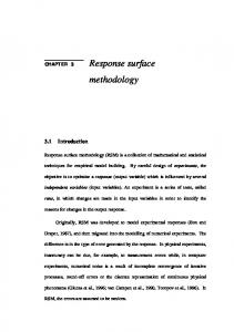
Configuration design variables Parallel simple aerodynamic analyses Parallel simple structural analyses Approximation domain Regression Analysis Response surface model structures D−optimal point selection D−optimal design point sets Aerodynamic Parallel structural Parallel detailed loads optimizations aerodynamic analyses Accurate aerodynamic Accurate quantities weights Aerodynamic response Weight response surfaces surface Configuration optimization Approximate optimal design
OPTIMAL DESIGN
Figure 1. General �ow chart for HSCT design. This study focuses on applying a variable-complexity response surface approximation strategy to HSCT design optimization. The simple analysis methods are used to de�ne a subregion of the design space, i.e., the approximation domain, in which an optimal HSCT design is likely to exist. The re�ned analysis methods are then used to construct smooth response surface models of various aerodynamic and structural weight quantities which are susceptible to numerical noise. Aerodynamic response surface models were constructed for volumetric wave drag and supersonic drag due to lift for an example wing design problem involving four of the twenty-eight HSCT design variables. A structural response surface model was also investigated for the wing bending material weight factor for a problem involving twenty-�ve of the HSCT design variables. The objective of the optimization procedure is to minimize the gross takeo� weight of the vehicle subject to numerous geometric, aerodynamic and performance constraints. Additional constraints limit the scope of the design space to the region over which the
Variable-Complexity Response Surface Design
3
response surface models are valid. Currently, the aerodynamic response surface models have been incorporated into the optimization strategy. However, we have not yet implemented the structural response surface models into this framework. A �ow chart illustrating the HSCT design process is given in Figure 1.
2 Variable-Complexity Modeling
We have termed \variable-complexity modeling" the design process by which simple, computationally inexpensive analysis techniques are used together with more detailed, expensive techniques. Originally, this methodology was developed for gradient-based optimization in which the overall design process was composed of a sequence of optimization cycles. With this method, the detailed analyses were employed at the beginning of each optimization cycle while the simple analyses, scaled to match the initial detailed results, were performed in subsequent calculations during each cycle �8], �22]. A typical HSCT design optimization requires approximately twenty cycles until an optimal HSCT con�guration is identi�ed. The optimizer NEWSUMT-A �13], which employs an extended interior penalty function method, is used for this sequential approximate optimization process. In the present work, this variable-complexity modeling approach is adapted for use with response surface approximation techniques. Here, the simple analysis methods are used to evaluate thousands of di�erent HSCT con�gurations within a prescribed design space. By applying constraints to the design variables and to the objective function data, \nonsense" regions of the design space are excluded. The valid design space is characterized by an irregularly shaped region which contains the optimal HSCT con�guration. Using a large number of points which span the valid, but irregularly shaped, design space, a small number of points, on the order of �fty to one hundred, are then selected for more detailed analyses. Using the results from these detailed analyses, response surface approximations can be created to model various factors which a�ect the HSCT design. For example, drag component data from the detailed analyses can be used to create a polynomial response surface model for the variation in drag. In the �nal step of this process, the response surface models are implemented in the HSCT analysis software, and con�guration optimization is carried out. This optimization uses constraints based on both the simple and detailed analyses, along with constraints which limit the design variables to values for which the response surface model is accurate.
3 Response Surface Methods 3.1 Polynomial Modeling
Response surface methodology (RSM) is a statistical technique in which smooth functions, typically polynomials, are used to model an objective function. For example, a quadratic response surface model for p design variables has the form: X X (1) y = co + ci xi + cij xixj + � 1�i�p
1�i�j �p
where the xi are the design variables, the ci are the polynomial coe�cients, y is the measured response, and is a random error term. In such a model the polynomial coe�cients may be estimated using the method of least squares. The construction of a response surface requires a minimum of n function evaluations where n is the number of coe�cients in the polynomial. Results from �12] con�rmed that
4
Giunta et al.
typically 1:5n function analyses were required to produce response surfaces which accurately approximated the global trends of the objective function data. An example of the use of response surface modeling techniques is provided in �12] where supersonic drag due to lift of an HSCT wing was calculated for various inboard leading-edge and inboard trailing-edge sweep angles. Here, drag due to lift is calculated as � 1 C T CDlift = C ; kt 2 CL2 � (2) L
CL
where CL is the lift curve slope, CT =CL2 is the leading-edge thrust term, and kt is an attainable leading-edge thrust factor. Numerical noise in the evaluation of drag due to lift (Fig. 2) may be attributed to noise in the lift curve slope and leading-edge thrust terms. The methods of Carlson et al. �5], �6], �7] utilize a paneling scheme that is sensitive to planform changes. Thus, slight modi�cations to the leading and trailing-edge sweep angles, along with changes in the location where the Mach angle intersects the leading-edge, produce discontinuous variations in the predicted drag. Although the variations are small enough so that at all points the accuracy of the drag is acceptable, the oscillatory behavior creates di�culties for gradient-based optimization techniques. Nonsmooth behavior of an objective function was also encountered in a nozzle design problem �25] in which an Euler �ow solver was employed indicating noisy or nonsmooth behavior is not solely related to the use of panel methods. Trailing−edge Sweep Angle (deg.) 50 2
CD(lift)/CL^2
25
CD(lift)/CL
0 0.58 0 0.57 0 5 0.57 0 0 0.56 0 5 0.56 0 0 0.55 0 50
0.6 0 0.59 0 0 0.58 0.57 0 0.56 0 0.55 0.
-25 -50
wee p (deg Angle .)
we (d ep A eg .) ngle
L.E .S
T. E. S
76 .0 76 .5 77 .0 77 .5 78 .0 78 .5 79 .0
60 40 . 0 20.0.0 0.0 -20 -40. .0 -60. 0 0
Figure 2. Noisy drag due to lift.
75 76 77 78 79 80 Leading−edge Sweep Angle (deg.)
Figure 3. Quadratic polynomial response surface �t to the noisy drag due to lift data.
Figure 3 demonstrates the use of a quadratic polynomial response surface to approximate the noisy drag due to lift in Figure 2. The global minimum on the exact, noisy surface occurs for a leading-edge sweep angle of 77:6� and a trailing-edge sweep angle of ;20:0�: As shown in Figure 3, the quadratic response surface provides a reasonable estimation for the location of the global minimum.
Variable-Complexity Response Surface Design
5
3.2 D-optimal Point Selection
RSM typically employs a structured method such as central composite design (CCD) for selecting analysis points in the design space �23]. However, CCD is meant for use with regularly shaped design spaces and not the irregularly shaped design spaces that will arise in this design problem. Further, CCD is not a practical point selection method for design problems with a large number of variables. In a previous study �12], it was found that the D-optimal criterion �3] provided a rational means for choosing any number of points within an irregularly shaped design space. The D-optimal criterion arises from the linear model Y � Xc, where Y is an m by 1 vector of objective function values, c is a k by 1 vector of coe�cients to be estimated, and X is an m by k matrix of constants having rank k. The rows of the matrix X are the response surface basis functions evaluated at the design points. For this system, the least squares estimate of c is c^ = (XT X);1 XT Y: The goal is to �nd the m points from a set of l > m candidate points existing in the design space that will yield the best �delity between the polynomial model and the actual objective function. The D-optimality criterion states that the m points to choose are those which maximize the determinant jXT Xj. Several relevant properties of this criterion are: 1. the set of points that maximizes jXT Xj is also the set of points that minimizes the maximum variance of any predicted value of the objective function, 2. the set of points that maximizes jXT Xj is also the set of points that minimizes the variance of the parameter estimates, 3. the design ;obtained is invariant to changes in scale. � There are ml = l!=(m!(l ; m)!) combinations of m points from the set of l candidate points which is often a very large number. For example, a small problem in two design variables may be to pick twenty-�ve points from 121 possible points (discretizing the design domain into ten sections in both directions leads to an 11 � 11 mesh). This leads to a total of 5:26 � 1025 possible combinations, one or more of which are D-optimal. Because pf the large number of combinations, a genetic algorithm was developed to e�ciently �nd a set of D-optimal points. In addition, the genetic algorithm allows D-optimal point selection for a design space of arbitrary shape.
3.3 Regression Analysis and ANOVA
When using RSM the designer often encounters what has been termed the \curse of dimensionality" in which the number of analysis points needed to construct a response surface model greatly increases as the number of design variables becomes large. For this reason, it would be advantageous if less signi�cant terms in the response surface model could be eliminated. Fortunately, there is a statistical technique, analysis of variance (ANOVA), which enables the less signi�cant terms in the polynomial approximation to be identi�ed. ANOVA involves estimating the variance of the predicted polynomial coe�cients and uses the variancecovariance matrix (XT X);1 : The diagonal terms in this square matrix, �i 2 � multiplied by Var( )� the variance in the objective function values Yi � are the variances of the respective coe�cients, ci � in the response surface polynomial model. The coe�cient of variation, V� for each term in the polynomial is calculated as ( p 100j� j Var(�) � c 6= 0� i (2) V= c 100� ci = 0, i
i
6
Giunta et al.
where the factor of 100 expresses the coe�cient of variation as a percentage. The term Var( ) is usually estimated by the RMS error of the least squares approximation at the m data points. A common approximation for this term is: (3) Var ( ) = ERMS 2 m=(m ; n)� where m is the number of points used in the least squares method, n is the number of terms in the model equation, and ERMS is the RMS error calculated using the di�erence between the response of the model equation and the data used for the least squares problem.
4 HSCT Design Problem
Successful aircraft con�guration optimization requires a simple, yet meaningful mathematical characterization of the geometry. We have developed a model that completely de�nes the HSCT design problem using twenty-eight design variables. Twenty-�ve of the design variables describe the geometry of the aircraft and can be divided into �ve categories: wing planform, airfoil shape, tail areas, nacelle placement, and fuselage shape. The wing planform is described using the root and tip chord lengths, the wing span, and by blending linear line segments at the leading and trailing edges. The wing planform geometry is depicted in Figure 4. The airfoil sections have round leading edges and are de�ned using an analytic description incorporating the following four design variables: the location of maximum thickness-to-chord (t=c) ratio for all airfoil sections, and the t=c ratios at the root chord, leading-edge break, and tip chord. The horizontal and vertical tail areas are described by two variables. The nacelles are �xed along the trailing-edge of the wing with a twenty-�ve percent overhang, and two variables de�ne their spanwise locations. The axisymmetric fuselage requires eight variables to specify both the axial positions and radii of the four fuselage restraint locations. Details of the geometry speci�cation appear in References �19] and �21] and the design variables are listed in Table 1.
(x2, x3)
x1
x6
(x4, x5)
x8 x7
Figure 4. Planform variable de�nition for the HSCT wing.
Variable-Complexity Response Surface Design
Num. Value 1 2 3 4 5 6 7 8 9 10 11 12 13 14
181.48 155.9 49.2 181.6 64.2 169.5 7.00 75.9 0.40 3.69 2.58 2.16 1.80 2.20
7
Table 1. HSCT design variables and baseline values. Description Num. Value Description Wing root chord, (ft) 15 1.06 Fuselage restraint 1, r (ft) LE break point, x (ft) 16 12.20 Fuselage restraint 2, x (ft) LE break point, y (ft) 17 3.50 Fuselage restraint 2, r (ft) TE break point, x (ft) 18 132.46 Fuselage restraint 3, x (ft) TE break point, y (ft) 19 5.34 Fuselage restraint 3, r (ft) LE wing tip, x (ft) 20 248.67 Fuselage restraint 4, x (ft) Wing tip chord, (ft) 21 4.67 Fuselage restraint 4, r (ft) Wing semi-span, (ft) 22 26.23 Nacelle 1, y (ft) Chordwise max. t=c location 23 32.39 Nacelle 2, y (ft) LE radius parameter 24 322,617 Mission fuel, (lbs) Airfoil t/c at root, (%) 25 64,794 Starting cruise altitude, (ft) Airfoil t/c at LE break, (%) 26 33.90 Cruise climb rate, (ft=min) Airfoil t/c at tip, (%) 27 697.9 Vertical tail area, (ft2 ) Fuselage restraint 1, x (ft) 28 713.0 Horizontal tail area, (ft2 )
The design problem is to minimize the takeo� gross weight of an HSCT con�guration with a range of 5,500 nautical miles and a cruise speed of Mach 2.4 while transporting 250 passengers. For this mission, in addition to the geometric parameters, three variables de�ne the idealize cruise mission (Table 1). One variable is the mission fuel and the other two are initial cruise altitude and the constant climb rate used in the range calculation. In this study, a baseline HSCT is used for comparison purposes and to provide a rough approximation to the center of the feasible design space. The baseline geometry is from an optimal HSCT con�guration previously investigated by members of our research group at Virginia Tech (Table 1) �8].
Num. 1 2 3-20 21 22 23 24 25 26 27-31 32 33 34
Table 2. Constraints on the HSCT design.
Geometric Constraint
Fuel volume � 50% wing volume Spike prevention Wing chord � 7.0 ft LE break � semi span TE break � semi span Inboard TE sweep > 0 deg Root chord t/c > 1.5% LE break chord t=c > 1.5% Tip chord t=c > 1.5% Fuselage restraints, x, in order Nacelle 1 outboard of fuselage Nacelle 1 inboard of nacelle 2 Nacelle 2 inboard of semi-span
Num. Aero. & Perform. Constraint 35 36 37-55 56 57-60 61 62 63 64 65 66
Range � 5,500 nmi CL at landing speed � 1 Section Cl at landing speed � 2 Landing angle of attack � � 12� Engine scrape at landing Wing tip scrape at landing Rudder de�ection � 22.5� Bank Angle � 5� Tail de�ect. for approach � 22.5� Takeo� rotation to occur � Vmin Engine-out limit with vertical tail
Sixty-six constraints which include geometry, performance, and aerodynamic constraints are included in the optimization �8]. The aerodynamic and performance constraints can only be assessed after a complete analysis of the HSCT design� however, the geometric constraints can be evaluated using algebraic relations based on the twenty-eight design
8
Giunta et al.
variables. For this reason, they o�er an e�cient means of narrowing the feasible design space. The geometric, performance and aerodynamic constraints are listed in Table 2.
5 Four Design Variable Aerodynamic Design of the HSCT Wing The detailed aerodynamic analyses use the Harris program for the supersonic volumetric wave drag �14], a Carlson Mach-box type method for supersonic drag-due-to-lift �6], �7], and a vortex-lattice program for landing performance. As part of our variable-complexity modeling approach we also employ simple aerodynamic analysis methods which are typically algebraic relations, and which require at least an order of magnitude less computational time than the associated detailed analysis methods. Details of each calculation are given in �21]. Compared to modern computational �uid dynamics tools, the detailed and simple analysis models used in this study are relatively inexpensive. However, the computational expense of using these methods quickly becomes substantial when they are employed in design optimization where the same calculation may be repeated thousands of times.
5.1 Wing Design Variables To develop and test the variable-complexity response surface optimization strategy we decided to construct an example problem involving only a few variables. For this reason, a four variable wing design problem was chosen. Here, two of the original planform variables, root chord and tip chord, were selected along with two new design variables (Fig. 5). The �rst new design variable was the inboard leading-edge sweep angle which was calculated from the original planform variables x2 and x3 : The second new variable is a constant scaling factor, �� by which the three t=c ratios from the HSCT baseline were modi�ed. For example, (t=c)root�new = � (t=c)root�baseline , (t=c)break�new = � (t=c)break�baseline , and (t=c)tip�new = � (t=c)tip�baseline , for 0:8 � � � 1:2: Thus, this new variable, �� replaces the three t=c ratio design variables used in the original HSCT wing parameterization. In addition to the new variable de�nitions, planform variables x4 and x5 were eliminated so that the trailing edge of the wing was straight. Further, in this simpli�ed model the span was held �xed. Variations in the root chord have a signi�cant e�ect on both the structural weight of the wing and on the volume available within the wing for fuel storage. These characteristics directly in�uence the gross weight of the HSCT. Perturbations in the leading-edge sweep and the t=c scaling factor primarily a�ect supersonic drag due to lift and the volumetric wave drag. Thus, the range and gross weight of the HSCT are a�ected through variations in the drag components.
Variable-Complexity Response Surface Design
2.
1. Croot
9
Λle inboard 4. thickness/chord scale factor on entire wing
3.
Ctip
Figure 5. Wing design variable de�nition for the four variable problem. The tip chord variable was selected speci�cally because it has only a minor impact on the weight and performance of the HSCT. For this reason, it was expected that the regression analysis and analysis of variance techniques would identify as negligible some of the response surface terms involving tip chord. This was con�rmed by the analysis results and is discussed below. Note that although the tip chord is a relatively unimportant design variable for this example problem and the analysis methods used, the aerodynamics of the wing tip region can strongly in�uence the design of a particular aircraft. Therefore, the tip chord is not a design variable that can be ignored. The design space for this four variable problem was determined by allowing the root chord and tip chord to vary �20 percent from the values on the baseline HSCT. The t=c scaling factor also varied �20 percent from a nominal value of unity. The leading-edge sweep was allowed to range only �9 percent from its baseline value. Variations in the sweep angle outside of this range produced con�gurations which were not realistic.
5.2 Design Space Reduction
The �rst stage in the variable-complexity response surface modeling process was to evaluate numerous HSCT designs using simple algebraic analysis methods. This was performed by discretizing the design space using a 6 � 6 � 6 � 6 uniform coarse grid, i.e., each design variable had six discrete values. The 1,296 (64 ) con�gurations de�ned by the combinations of the design variable values were then analyzed. At the center of the design space was the baseline HSCT con�guration. Using the constraint data obtained for each of the 1,296 HSCT designs, obvious \nonsense" con�gurations were eliminated from consideration. Here, designs were excluded if any of the aerodynamic/performance constraints (e.g., landing angle-of-attack � 12�) were violated by more than twenty percent, and if any geometric constraints (e.g., minimum airfoil chord lengths � 7 ft.) were violated by more than �ve percent. In addition, gross
10
Giunta et al.
takeo� weight (GTOW) was allowed to vary within �20 percent of the baseline GTOW of approximately 650,000 lbs. and range was required to be greater than 5,000 n:mi: Both of these constraints were imposed to remove from consideration any unrealistic designs which had not been eliminated previously. After applying these constraints, only 157 acceptable HSCT designs remained out of the initial 1,296 designs.
5.3 Regression Analysis and ANOVA
Since range is directly a�ected by numerical noise in the supersonic drag due to lift and volumetric wave drag calculations, a response surface model for range was used to determine the reduced-term polynomial model for the D-optimal point selection and for later use in modeling the drag components. An alternative approach, and one that will be considered in our future work, would have been to apply regression analysis and ANOVA separately to response surface models for each of the drag components. With the data from the 157 simple HSCT analyses a �fteen term polynomial response surface model was �t to the aircraft range data. Using the regression analysis and ANOVA methods described above, the coe�cients of variation for the �fteen terms in the response surface model were calculated (Table 3). Here, the abbreviations �� cr � ct � and �LE correspond to the t=c scaling factor �� root chord, tip chord, and leading-edge sweep angle, respectively. As shown, the higher order terms involving ct have coe�cients of variation greater than ten percent and can safely be dropped from the response surface model. Thus, the number of terms in the response surface model was reduced to eleven and the modeling of the tip chord variable was simpli�ed from quadratic to linear. Table 3. Regression analysis and ANOVA data for the range response surface model.
Variable Coe�. Std. Dev const: cr �LE � ct cr ct ct �LE cr 2 �LE 2
0.058 -0.555 0.755 0.009 -0.025 -0.021 -0.147 -0.107
0.197 0.206 0.261 0.372 0.290 0.358 0.352 0.700
V
3.416 0.372 0.346 40.616 11.621 16.955 2.399 6.526
Variable �
ct
� cr
� �LE cr �LE �2
ct 2
Coe�. Std. Dev -1.200 -0.054 -0.221 0.170 0.058 -0.095 -0.006
0.268 0.133 0.627 0.848 0.572 0.623 0.234
V
0.224 2.443 2.835 4.990 9.907 6.588 42.143
The accuracy of the response surface �t is only slightly impaired after removing terms from the polynomial model for which the coe�cient of variation was large. With all �fteen terms in the polynomial, the average error (in nautical miles) was 11.71, the RMS error was 14.99 and the maximum error was 43.13. Removing four terms from the original polynomial brought the average error to 11.98, the RMS error to 15.45 and the maximum error to 38.61. Here, the errors are calculated from the di�erence between the response surface prediction for the range and the actual value for the range at each of the 157 remaining HSCT design points. From the 157 HSCT designs, �fty were selected on the basis of the D-optimal criterion. The performance and constraint criteria for each of these were then evaluated using the detailed aerodynamic analysis models. Using the same eleven term polynomial model found for range, new response surface models were constructed for the wave drag, the lift curve slope, and the leading-edge thrust term. These three response surface models were then used in the range calculation subroutine in place of the original noisy calculations of the drag components.
Variable-Complexity Response Surface Design
11
5.4 Optimization Techniques
As described above, the optimization for the variable complexity response surface approximation method uses constraints based on both the simple and detailed analysis models. For the example problem, this is accomplished by using two constraints on the calculated range. The approximate constraint uses the original range calculation, i.e., range calculated from the simple analysis of drag components, which must be greater than 5,000 n:mi: This is the same constraint used to remove unrealistic design points after the initial 1,296 HSCT analyses. The new range constraint employs the smooth response surface models for the three drag components. This constraint stipulates that the range must be greater than 5,500 n:mi: The complication is that the range based on the response surface models is accurate only for certain regions of the design space de�ned by the allowable design variable values. One may picture the response surface models as being valid on a four-dimensional spheroid inscribed within a four-dimensional hypercube, where the vertices of the hypercube are de�ned by the allowable limits on the design variables. Without the approximate range constraint � 5,000 n:mi:, the optimizer invariably moves to a vertex of the hypercube outside of the spheroid on which the response surface models are valid. At �rst this seems counterproductive since two constraints are now used for range whereas only one su�ced before. However, this arrangement circumvents the problems created by numerical noise in the original range constraint evaluation. The use of both approximate and response surface based range constraints is successful because the simple, noisy range constraint is not active for much of the optimization. It serves only to keep the optimizer from moving to a region of the design space where the response surface model is inaccurate. In contrast, the response surface based smooth range constraint is nearly always active but it is not a�ected by numerical noise. Due to improvements and corrections in various elements of our HSCT analysis software, the previously feasible baseline HSCT con�guration, was found to slightly violate several constraints. In particular, these violated constraints pertained to takeo� and landing conditions regarding wing tip/runway scrape, engine/runway scrape, and landing angle-of-attack. Since span was not a design variable in this example problem, some of these constraints would have remained violated for all combinations of the four design variables. Therefore, to complete this investigation, the constraints in violation were removed, and the landing angle-of-attack constraint was relaxed from 12� to 13�: With the HSCT baseline con�guration now providing a feasible starting point, optimization cases both with and without the response surface models for drag were conducted.
5.5 Optimization Results
With the range constraint based on the response surface models for volumetric wave drag and the two components of supersonic drag due to lift, the NEWSUMT-A optimizer was used to determine the optimal combination of wing design variables to yield minimum gross weight while satisfying all constraints. The results of the optimization are shown in Table 4 in which the design variables and performance are compared for the initial and optimal HSCT con�gurations. Figure 6 shows the di�erence between the baseline HSCT planform from which the optimization was started and the optimal planform. The planform changes
12
Giunta et al.
for the optimal wing design are most noticeable in the length of the root chord and in the leading-edge sweep angle. However, these di�erences are relatively modest. Table 4. HSCT performance data for the initial and optimal HSCT designs.
root chord tip chord LE sweep t/c scale
Initial
174.0 ft: 8.1 ft: 71.88� 1.00
Exact Range 5,577 n:mi: R.S. Range 5,546 n:mi: Landing AOA 12.28�
Optimal 171.1 ft: 7.8 ft: 72.44� 0.92
5,510 n:mi: 5,519 n:mi: 12.33�
Wing Weight Fuel Weight GTOW Fuel/Gross
CDwave
Total Drag
Initial
Optimal
0.0017 0.0053
0.0015 0.0052
107,410 lbs: 103,123 lbs: 328,044 lbs: 310,750 lbs: 643,393 lbs: 620,876 lbs: 50.99 % 50.05 %
The thinner wing results in a lower wave drag coe�cient and thus a lower total drag coe�cient. This improvement in aerodynamic e�ciency permits the elimination of 18,000 lbs: of unneeded fuel. Additional weight savings occur because the optimal wing is smaller. Speci�cally, the wing area has decreased by 5.5 percent. Although the optimal wing is thinner, and therefore requires a heavier structure, the weight penalty is o�set by the decrease in wing size. Thus, the optimal wing design results in a combined weight reduction of approximately 22,500 lbs:, which is a 3.5 percent decrease in GTOW. For comparison, the optimization of the four variable design problem was repeated, but without using the response surface models for the drag components. In this case the sequential approximate optimization strategy was applied. The result of this optimization yielded a nearly identical optimal design as was obtained using the optimization with the response surface models. Di�erences in the optimal design variables and in the analysis results were negligible. Distance along Fuselage (ft.) 0.0
-50.0
Baseline HSCT Planform Optimal HSCT Planform
-100.0
-150.0
-200.0 0.0
50.0 100.0 150.0 200.0 Distance from Fuselage Centerline (ft.)
Figure 6. Baseline vs. optimal HSCT planforms. In this case, the optimizer also found the minimum design after one sequential approximate optimization cycle. However, this was not unexpected since the baseline HSCT design was very close to an optimal design. In general, the optimal design will not be near the initial HSCT design and experience has shown that the sequential approximate optimization
Variable-Complexity Response Surface Design
13
strategy will require approximately twenty global optimization cycles until convergence is reached.
6 Wing Structural Weight Estimation
Gross takeo� weight is minimized during the HSCT con�guration optimization process. Therefore, weight calculations are numerous and the �nal HSCT design is highly dependent on the accuracy of these results. To ease the computational expense of the design process, we have implemented the statistical weight equation in the weight module of Flight Optimization System (FLOPS) �24]. FLOPS is used to determine take-o� gross weight and, more specially, to �nd the e�ect of planform geometry changes on structural weight. However, since the HSCT is a new aircraft, the weight equation does not account for all features of the design. Because of the limitations within FLOPS, we have looked to improve upon the accuracy of the structural weight predictions. In particular, we have focused on the wing bending material weight since most of the load-dependent wing weight is due to bending.
6.1 The Weight Equation
The general wing weight equation in FLOPS is based on an analytic expression to relate wing bending material weight to wing geometry, material properties and loading. Other terms are added to account for shear material, control surfaces, etc. In addition, constants are included to correlate with a wide range of existing transports and re�ect features such as composite materials, strut braced wings, etc. The wing weight, Ww , used within FLOPS is given as (4) Ww = Wg Ke W1b++WWs + Wn � b where Ws = 0:68 (1 ; 0:17fc) (S ; Sb )0:34 Wg0:6 � Wn = 0:35 (1 ; 0:3fc ) S 1:5 � Wb = Kful b (1 ; 0:4fc) (1 ; :01fa) � � � K = 8:8Bz 1 + (6:25=b)0:5 � 10;6 � Ke = 1:0 ; (Bze =Be ) (Wpod=Wg ) � and Wg is the gross take-o� weight (lbs), Wb is the wing bending material weight (lbs), Ws is the wing shear material and �aps weight (lbs), Wn is the wing control surfaces and nonstructural weight (lbs), Wb is the wing bending material weight (lbs), Wpod is the engine pod weight (lbs), b is the wing span (ft), Bz is the bending material factor, Bze is the engine relief factor, ful is the ultimate load factor, fa is the composite material factor, fc is the aeroelastic tailoring factor, S is the wing area (ft2 ), and Sb is the wing box area (ft2 ). The FLOPS wing weight calculation is an iterative process since the wing weight and the gross take-o� weight are dependent on one another. The system is closed except for the bending material factor, Bz , and the engine relief factor, Bze . Bz accounts for the load distribution on the wing and is calculated by approximately determining the required material volume of the upper and lower skins in a simple wing box description of the wing. Bze accounts for the reduced amount of structural weight necessary due to the presence of the engines on the wing.
14
Giunta et al.
6.2 Response Surface Approximation to Weight Equation
Finite-element based structural optimization appears to be an e�ective way to improve the estimate for the wing bending material weight given by FLOPS. However, �nite-element solutions do not produce smooth functions with respect to the design variables. Thus, gradient-based optimizations are di�cult to perform. In addition, the computational expense of �nite-element solutions prevents them from being used frequently within the HSCT design optimization process. For these reasons, we have turned to a response surface approximation of the wing bending material weight. This provides a simple algebraic means of calculating accurate values for the wing bending material weight while at the same time giving smooth derivative information. In the development of the response surface, a large number of data points, which span the design space, are required� however, we are limited by the expense of performing structural optimizations. For this reason, the wing bending material weight predicted by FLOPS will be used to develop the response surface. Once this is done, a sequence of structural optimizations will be performed using �nite element analysis to generate the �nal form of the response surface.
6.3 The Model Equation
To determine a generalized model equation, we looked at the basic form of statistical weight equations such as those de�ned within FLOPS. A basic algebraic relationship which appears repeatedly is: (5) y = Cxc11 xc22 � � � xcn � where y is the objective function and x are the variables. From this a generalized model equation can represented as: X X (6) ln(y ) = co + 1 � i � pci ln (xi ) + cij ln (xixj ) + � n
p
1�i�j �p
Essentially, the logarithm of the response, y , is a function of a quadratic in the logarithms of the variables, x. The ci coe�cients are unknown values which must be found through the method of least squares.
6.4 Identi cation of the Feasible Design Space
For simplicity, we initially chose the variables to be twenty-�ve of the twenty-eight HSCT design variables. The remaining three variables, the wing leading edge radius, the cruise climb rate and the starting cruise altitude were neglected because they had no e�ect on the wing bending material weight. The enormous design space associated with the twenty-�ve variables, as well as the expense of performing structural optimizations, forced us to limit the response surface to feasible regions of the space. Therefore, the �rst step in the response surface design was to �nd a large group of candidate points in the feasible region. Initially, we found a twenty-�ve dimensional hypercube which encompassed the entire feasible region. This was accomplished by allowing each of the variables to assume values between 20 percent and 180 percent of their baseline value, given in Table 1. In this response design space, 19,651 con�gurations were found distributed evenly throughout the hypercube. Of these designs, 83 percent violated one or more of the HSCT geometric constraints. Using a simple search method, each of the geometrically infeasible con�gurations
Variable-Complexity Response Surface Design
15
was moved into the feasible region of the design space by moving the design a distance � closer to the baseline con�guration. (7) x0 = � (x ; xc) + xc x0 is the transformed point based on x while xc is the baseline value discussed previously. To further limit the extent of the design space, obvious nonsense designs were removed based on the wing bending material weight predicted by FLOPS. Values below 20,000 lbs: or above 120,000 lbs: were considered unreasonable and excluded from the set of candidate points. Thus, we were left with 18,152 feasible designs.
6.5 Selection of Intervening Variables
Using the initial twenty-�ve variables and the 18,152 design points, a response surface model was �t to wing bending material weight estimates from FLOPS. The accuracy of this response surface, however, was found to be unacceptable. The average error was 952 lbs:, the RMS error was 2,895 lbs:, and the maximum error was 196,576 lbs: Errors were calculated from the di�erence between the response surface predictions for the wing bending material weight and the values predicted by FLOPS. One method to �nd a more accurate response surface would be to use the same variables in conjunction with another form of the model equation. However, the quadratic equation was already very general and moving to a more general equation, like a cubic, would signi�cantly increase the complexity of the model equation. For this reason we chose to �nd an alternative set of variables, intervening variables, which would be more appropriate for a weight analysis while also being entirely dependent on the design variables. Compared to the original variables, properly chosen intervening variables can produce accurate results using a less complex model equation. Returning to the description of the FLOPS weight equation, the wing weight is based on a set of ten basic parameters. Listed in Table 5, each of these parameters can be found using the twenty-�ve HSCT design variables. Using these terms as the intervening variables produced dramatically better results. The average error was 17 lbs:, the RMS error was 47 lbs:, and the maximum error was 1,345 lbs: Table 5. Basic parameters used to calculate wing weight in FLOPS.
Num. Name 1 2 3 4 5
Sht Svt wfuse b sweep
Description
Horiz. tail area Vert. tail area Max. fuselage diam. Wing span Ave. 1=4 chord sweep
Num.
6.6 Regression Analysis and ANOVA
6 7 8 9 10
Name Bze Bz Sw Wfuel Wto
Description
Engine relief factor Bending material fact. Wing surface area Takeo� fuel weight Gross weight from FLOPS
The FLOPS weight equation was used to �nd the wing bending material weight for the 18,152 designs. Using these values as the objective function and the ten intervening variables discussed previously, regression analysis and analysis of variance (ANOVA) methods were used to �nd the coe�cients of variation for each of the sixty-six terms in the model equation. The non-linear terms with the lowest coe�cient of variation were then removed from the model equation, and the process of regression analysis and ANOVA was repeated.
16
Giunta et al.
Figure 7 shows the accuracy of the response surface compared to the number of terms remaining in the model equation. Reducing the complexity of the model equation by fortyone terms had only a minor impact on the accuracy. This twenty-�ve term model equation was chosen for further analysis. 100
140
RMS Error Average Error
RMS Error 120
Average Error
100
60
Error (pounds)
Error (pounds)
80
40
80
60
20 40
0 10
20
30
40
50
Terms in Model Equation (Maximum 66)
60
70
20 0
50
100
150
200
Number of Points
Figure 7. RMS Error versus terms Figure 8. Comparison of the twenty-�ve remaining in the model term model equation accuracy equation. using D-Optimal points. Up to this point, all 18,152 con�gurations had been used to construct the response surface. However, the expense of structural optimizations severely limits the number of designs which can be considered. To address this issue, several subsets of the 18,152 points were identi�ed using D-optimality �3]. The accuracy of the model equation versus the number of design points used is given in Figure 8. As with the number of terms in the model equation, the number of points required to produce an accurate response surface is signi�cantly less than the original 18,152 points. From Figure 8, it appeared that sixty con�gurations would produce an accurate response surface based on the twenty-�ve term model equation.
6.7 Structural Optimization
The structural optimization procedure minimizes the weight for a given �xed arrangement of the spars and ribs with the thicknesses of skin panels, spar and rib cap areas as design variables. Von Mises stress constraints are applied to all the panel, spar, and rib cap elements. Local buckling constraints are also applied. Creating a response surface requires numerous planform evaluations. For this reason, a special mesh generator was implemented to automatically create a �nite element model based on the 28 HSCT design variables. In addition to design variables, the number of frames in the fuselage, the number of spars and ribs in the wing and the chord fractions taken by the leading and trailing edge control surfaces must be speci�ed. The mesh generator creates the �nite element nodes and element topology data in addition to estimating the location of non-structural weights and the geometry of the wing fuel tanks �17]. A typical �nite element model is made up of 923 elements joined at 193 nodes with 579 total degrees of freedom. The wing and fuselage skin are modeled by membrane elements. Spar and rib cap elements are modeled by rod elements. Vertical rods and shear panels are used to model spar and rib webs. The initial thicknesses and areas of the elements were chosen to match the estimated structural weight. The aircraft is assumed to be built of titanium. Because of symmetry, only half of the aircraft was modeled.
Variable-Complexity Response Surface Design
17
The loads applied to the structural model are composed of the aerodynamic forces and inertia forces due to the distributed weight of the structure, non-structural items and fuel. Aerodynamic loads for supersonic �ight conditions were determined using a supersonic panel method, and loads for subsonic �ight conditions were from a vortex-lattice method. Carlson's WINGDES program was used to generate a cambered wing from the given aerodynamic con�guration �5]. The loads at the aerodynamic nodes were mapped to the structural nodes using surface spline interpolation. The structure was assumed to be rigid for the determination of aerodynamic forces. (Previous studies indicated that structural �exibility did not have a large e�ect on the loads for this particular con�guration �1], �18].) The fuel was assumed to be stored in thirty-one tanks throughout the aircraft. More details about load cases used can be found in �20].
7 Parallel Computing 7.1 Parallel Implementation of Aerodynamic Analysis Our e�orts at parallel computing involve a twenty-eight node Intel Paragon at Virginia Tech. The coarse grained parallelization of the aerodynamic analysis modules within the full HSCT analysis code makes use of a master-slave paradigm on the Paragon whereby one designated master node controls the data transfer and �le input/output (I/O) of the remaining slave nodes. This coarse grained approach is used for the numerous independent analyses required for response surface construction. To initiate the parallel multipoint analyses, a group of predetermined analysis points is input to the master node. The master node then computes the subset of the points which each slave node will analyze and sends that information to the appropriate slave. Both the master and slave nodes then analyze their respective subsets of the selected points and store the results in an array local to each node. When each slave has �nished its portion of the analyses, it sends the array of analysis values to the master node for output. To compare the computational savings for parallel versus serial execution of a code, the term speedup is de�ned as Ts =Tp� where Ts is the serial execution time and Tp is the parallel execution time using p processors. Figure 9 shows the speedup results for parallel execution of the HSCT analysis code compared to ideal, linear speedup. The actual results deviate from the ideal due to the �le I/O demands of the analysis code which must be executed serially, and due to unavoidable communication overhead in the parallel code. Currently we are examining methods to reduce �le I/O and improve the parallel execution of the HSCT analysis code. Our e�orts to date are detailed in Reference �4].
18
Giunta et al. 25
Ideal
50
Ideal speedup
Simple Analysis 40
GENESIS, reduced I/O
15
30
Speedup
Speedup = Ts/Tp
GENESIS 20
Detailed Analysis
20
10
10
5
0 0
10
20 30 40 p, Number of Processors
50
Figure 9. Ideal versus actual speedup for parallel execution of the HSCT aerodynamic code.
0 0
5
10 Number of Processors
15
20
Figure 10. Ideal versus actual speedup for parallel execution of the GENESIS code.
7.2 Parallel Implementation of Structural Analysis
The repeated structural optimizations required to produce a response surface are suitable for coarse-grained parallel computation. Coarse-grained parallelization implies that multiple con�guration geometries will be evaluated simultaneously, each on a separate processor. There is no interaction between the processors, each maintaining their own input and output data. For a distributed memory architecture, disk I/O limits the e�ciency of the parallel computations as the number of processors are increased. This factor was the primary basis for choosing a particular structural optimization code to implement in the parallel environment. GENESIS, a �nite-element structural optimization code developed and supported by Vanderplaats, Miura and Associates, Inc �11], was available from the developer in a reduced I/O form and thus made it an e�ective code to use on the Paragon. With the standard version of GENESIS the maximum speedup level is 2.3 even with a large number of processors. The reduced I/O version achieves a speedup of 11.7 using twenty processors (Fig. 10).
8 Continuing Work
Currently the four variable HSCT wing design problem is being fully explored and the variable-complexity response surface modeling techniques are being re�ned. These methods will be applied to a new HSCT design problem involving seven to ten design variables to further validate the response surface modeling procedure. We have developed a model equation which has been found to be e�ective in predicting the wing bending material weight given by the FLOPS weight equation. Our future e�orts focus on evaluating the suitability of the model equation to data produced by GENESIS. This will be accomplished by performing numerous structural optimizations in parallel for a subset of the 18,152 planforms generated previously. The subset of points will be determined using the D-optimal criterion and the objective will be to �nd the minimum number of points required to produce an accurate response surface model. The �nal form of the response surface model, based on the �nite element structural optimizations, will be integrated into the HSCT design process. The algebraic response
Variable-Complexity Response Surface Design
19
surface model will replace the wing bending material weight term calculated using FLOPS. One problem which we anticipate will be identifying regions where the response surface is inaccurate. The optimizer may evaluate designs outside of the domain of validity for the response surface and would calculate erroneous values for the wing bending material weight. To circumvent this problem, an additional constraint will be added to the optimizer which will preclude HSCT designs where the FLOPS equation predicts a wing bending material weight outside of the range used to create the response surface. This �ts into the variable-complexity modeling strategy in that the inexpensive FLOPS evaluations are used in conjunction with the response surface models calculated from the GENESIS �nite element optimizations.
9 Concluding Remarks
A variable-complexity response surface modeling strategy has been developed and has been applied to the multidisciplinary design optimization of an HSCT. The feasibility of this method has been demonstrated using response surface models for aerodynamic drag components in a four variable HSCT wing design problem. Further, the response surface techniques have been applied to structural analysis in the development of a model for the wing bending material weight for various HSCT con�gurations. This structural model will be integrated into the overall HSCT design optimization framework. The combined variable-complexity aerodynamic and structural response surface methods will then be applied to the full HSCT design problem involving twenty-eight or more design variables. Additional e�orts will be directed at further improving the parallel performance of both the aerodynamic and structural analysis methods.
References
�1] Barthelemy, J. F. M., Wrenn, G. A., Dovi A. R., Coen, P. G., and Hall, L. E., Supersonic Transport Wing Minimum Weight Design Integrating Aerodynamics and Structures, J. of Aircraft, vol. 31, No. 2, March{April 1994. �2] Box, G. E. P. and Behnken, D. W., Some New Three Level Designs for the Study of Quantitative Variables, Technometrics, vol. 2, No. 4, November, 1960, pp. 455{475. �3] Box, M. J. and Draper, N. R., Factorial Designs, the jXT Xj Criterion, and Some Related Matters, Technometrics, vol. 13, No. 4, 1971, pp. 731{742. �4] Burgee, S., Giunta, A. A., Narducci, R., Watson, L. T., Grossman, B., and Haftka, R. T., A Coarse Grained Variable-Complexity Approach to MDO for HSCT Design in Parallel Processing for Scienti�c Computing, Bailey, D. H., Bj�rstad, P. E., Gilbert, J. R., Mascagni, M. V., Schreiber, R. S., Simon, H. D., Torczon, V. J., and Watson, L. T. (eds.), SIAM, Philadelphia, PA, 1995, pp. 96{101. �5] Carlson, H. W., and Mack, R. J., Estimation of Leading-Edge Thrust for Supersonic Wings of Arbitrary Planforms, NASA TP-1270, 1978. �6] Carlson, H. W., Mack, R. J., and Barger, R. L., Estimation of Attainable Leading-Edge Thrust for Wings at Subsonic and Supersonic Speeds, NASA TP-1500, 1979. �7] Carlson, H. W., and Miller, D. S., Numerical Methods for the Design and Analysis of Wings at Supersonic Speeds, NASA TN D-7713, 1974. �8] Dudley, J., Huang, X., MacMillin, P. E., Grossman, B., Haftka, R. T., and Mason, W. H., Multidisciplinary Optimization of the High-Speed Civil Transport, AIAA Paper 95{0124, 1995. �9] Dudley, J., Huang, X., Haftka, R. T., Grossman, B., and Mason, W. H., Variable-Complexity Interlacing of Weight Equation and Structural Optimization for the Design of the High Speed Civil Transport, AIAA Paper 94{4377, 1994.
20
Giunta et al.
�10] Engelund, W. C., Stanley, D. O., Lepsch, R. A., McMillin, M. M., and Unal, R., Aerodynamic Con�guration Design Using Response Surface Methodology Analysis, AIAA Paper 93-3967, Aug. 1993. �11] GENESIS, User Manual, Version 1.3, Dec. 1993. �12] Giunta, A. A., Dudley, J. M., Narducci, R., Grossman, B., Haftka, R. T., Mason, W. H., and Watson, L. T., Noisy Aerodynamic Response and Smooth Approximations in HSCT Design, AIAA Paper 94{4376, 1994. �13] Grandhi, R. V., Thareja, R., and Haftka, R. T., NEWSUMT-A: A General Purpose Program for Constrained Optimization Using Constraint Approximation, ASME J. Mechanisms, Transmissions and Automation in Design, vol. 107, 1985, pp. 94{99. �14] Harris, R. V., Jr., An Analysis and Correlation of Aircraft Wave Drag, NASA TM X-947, 1964. �15] Healy, M. J., Kowalik, J. S, and Ransay, J. W., Airplane Engine Selection by Optimization on Surface Fit Approximations, J. Aircraft, vol. 12, No. 7, 1975, pp. 593{599. �16] Hinkelman, Klaus., Design and Analysis of Experiments, John Wiley & Sons, Inc., 1994. �17] Huang, X., Structural Optimization and it's Interaction with Aerodynamic Optimization for a High Speed Civil Transport, Ph.D. Dissertation, VPI&SU, November 1994. �18] Huang, X., Haftka, R. T., Grossman, B., and Mason, W., Comparison of Statistical-based Weight Equations with Structural Optimization for Supersonic Transport Wings, AIAA 94{ 4379, 1994. �19] Hutchison, M. G., \Multidisciplinary Optimization of High-Speed Civil Transport Con�gurations Using Variable Complexity Modeling, Ph.D. Dissertation, VPI&SU, March 1993. �20] Hutchison, M. G., Huang, X., Mason W. H., Haftka, R. T., and Grossman, B., VariableComplexity Aerodynamic-Structural Design of a High-Speed Civil Transport Wing, 4th AIAA/USAF/NASA/OAI Symposium on Multidisciplinary Analysis and Optimization, Cleveland, OH, Sept. 21-23, 1992. �21] Hutchison, M. G., Unger, E. R., Mason, W. H., Grossman, B., and Haftka, R. T., Aerodynamic Optimization of an HSCT Wing Using Variable-Complexity Modeling, AIAA 93{0101, Jan. 1993. �22] Hutchison, M. G., Unger, E. R., Mason, W. H., Grossman, B., and Haftka, R. T., VariableComplexity Aerodynamic Optimization of an HSCT Wing Using Structural Wing-Weight Equations, J. Aircraft, vol. 31, No. 1, 1994, pp. 110{116. �23] Mason, R. L., Gunst, R. F., and Hess, J. L., Statistical Design and Analysis of Experiments,, John Wiley & Sons, New York, N. Y., 1989, pp. 215{221. �24] McCullers, L. A., Aircraft Con�guration Optimization Including Optimize Flight Pro�les, Proceedings of a Symposium on Recent Experiences in Multidisciplinary Analysis and Optimization, J. Sobieski, compiler, NASA CP{2327, April 1984, pp. 395{412. �25] Narducci, R., Grossman, B., and Haftka, R. T., Sensitivity Algorithms for an Inverse Design Problem Involving a Shock Wave, AIAA Paper 94-0096, Jan. 1994, to appear in Inverse Problems in Engineering. �26] Unger, E. R., Hutchison, M. G., Rais-Rohani, M., Haftka, R. T., and Grossman, B., VariableComplexity Design of a Transport Wing, Intl. J. Systems Automation: Res. and Appl. (SARA), No. 2, 1992, pp. 87{113.