Hindawi Publishing Corporation e Scientific World Journal Volume 2014, Article ID 274897, 10 pages http://dx.doi.org/10.1155/2014/274897
Research Article Variable Is Better Than Invariable: Sparse VSS-NLMS Algorithms with Application to Adaptive MIMO Channel Estimation Guan Gui,1 Zhang-xin Chen,2 Li Xu,1 Qun Wan,2 Jiyan Huang,2 and Fumiyuki Adachi3 1
Department of Electronics and Information Systems, Akita Prefectural University, Akita 015-0055, Japan Department of Electronic Engineering, University of Electronic Science and Technology of China, Chengdu 611731, China 3 Department of Communications Engineering, Tohoku University, Sendai 980-8579, Japan 2
Correspondence should be addressed to Guan Gui;
[email protected] Received 2 February 2014; Accepted 26 May 2014; Published 24 June 2014 Academic Editor: Serkan Ery´ılmaz Copyright © 2014 Guan Gui et al. This is an open access article distributed under the Creative Commons Attribution License, which permits unrestricted use, distribution, and reproduction in any medium, provided the original work is properly cited. Channel estimation problem is one of the key technical issues in sparse frequency-selective fading multiple-input multiple-output (MIMO) communication systems using orthogonal frequency division multiplexing (OFDM) scheme. To estimate sparse MIMO channels, sparse invariable step-size normalized least mean square (ISS-NLMS) algorithms were applied to adaptive sparse channel estimation (ACSE). It is well known that step-size is a critical parameter which controls three aspects: algorithm stability, estimation performance, and computational cost. However, traditional methods are vulnerable to cause estimation performance loss because ISS cannot balance the three aspects simultaneously. In this paper, we propose two stable sparse variable step-size NLMS (VSSNLMS) algorithms to improve the accuracy of MIMO channel estimators. First, ASCE is formulated in MIMO-OFDM systems. Second, different sparse penalties are introduced to VSS-NLMS algorithm for ASCE. In addition, difference between sparse ISSNLMS algorithms and sparse VSS-NLMS ones is explained and their lower bounds are also derived. At last, to verify the effectiveness of the proposed algorithms for ASCE, several selected simulation results are shown to prove that the proposed sparse VSS-NLMS algorithms can achieve better estimation performance than the conventional methods via mean square error (MSE) and bit error rate (BER) metrics.
1. Introduction High-rate data broadband transmission over multiple-input multiple-output (MIMO) channel has become one of the mainstream techniques for the next generation communication systems [1]. The major motivation is due to the fact that MIMO technology, as shown in Figure 1, is a way of using multiple antennas to simultaneously transmit multiple streams of data in wireless communications [2] and hence it can bring considerable improvements such as data rate, reliability, and energy efficiency. In fact, coherent receivers require accurate channel state information (CSI) since the received signals are distorted by multipath fading transmission. The accurate estimation of channel impulse response (CIR) is a crucial aspect and challenging issue in coherent
modulation and its accuracy has a significant impact on the overall performance of the communication system. During last decades, there exist many channel estimation methods which were proposed for MIMO systems [3–11]. All these methods are categorized into two groups. The first group contains the linear channel estimation methods, for example, least squares (LS) algorithm, based on the assumption of dense CIRs. By applying these approaches, the performance of linear methods depends only on the size of MIMO channel. Note that narrowband MIMO channel may be modeled as dense channel model because of its very short time delay spread. Accurately, broadband MIMO channel is often modeled as sparse channel model [12–14]. A typical example of sparse channel is shown in Figure 2. It is well known that linear channel estimation methods are
2
The Scientific World Journal
x1 Input signal
Output signal
Unknown MIMO channel
.. .
.. .
y1
∑
h1N𝑡 x
.. .
.. .
.. .
matrix H
h11 .. .
x N𝑡
hN𝑟 1 .. .
.. .
yN𝑟
∑
hN𝑟 N𝑡
Figure 1: Signal transmission over MIMO channel. ̃N : h 𝑟 .. .
0.7
̃ 1: h
Magnitude
0.6
−
+
−
+
0.5
eN𝑟 · · · e1
0.4
Adaptive algorithm
Figure 3: Adaptive algorithm for estimating MIMO channels.
0.3 0.2 0.1 0
0
5
10
15 Tap index
20
25
30
Number of overall taps: 32 Number of nonzero taps: 4
Figure 2: A typical example of sparse multipath channel.
relatively simple to implement due to their low computational complexity [3–8]. Unfortunately, their main drawback is the failure to exploit the inherent channel sparsity. The second group is the sparse channel estimation methods which use compressive sensing (CS) theory [15, 16]. Interested authors are recommended to refer to [17]. Basically, optimal sparse channel estimation often requires that its training signal satisfies restrictive isometry property (RIP) [18] in high probability. However, designing the RIP-satisfied training signal is a nonpolynomial (NP) hard problem [19]. Also, there exist some proposed methods which are stable with the cost of extra computational burden, especially in time-variant MIMO systems. For example, sparse channel estimation method using Dantzig selector was proposed for doubleselective fading MIMO systems [10]. Indeed, the proposed method needs to be solved by linear programming which incurs high computational complexity. To reduce the computational cost, sparse channel estimation methods using greedy iterative algorithms were also proposed in [9, 11]. But their complexity still depends on the number of nonzero taps of MIMO channel.
Unfortunately, the mentioned proposed methods do not have adaptive estimation capability. Adaptive sparse channel estimation (ASCE) methods using sparse invariable step-size (ISS) least mean square algorithms (ISS-LMS) were proposed in [20] for single-input single-output (SISO) channels. However, conventional ISS-LMS methods have two main drawbacks: (1) sensitive to random scale of training signal and (2) unstable in low signal-to-noise ratio (SNR) regime. To overcome the two harmful factors on channel estimation and extend their applications to estimate MIMO channels, sparse ISS normalized least mean square (ISS-NLMS) algorithms, for example, zero-attracting ISS-NLMS (ZA-ISSNLMS) and reweight ZA-ISS-NLMS (RZA-ISS-NLMS), were proposed in [21]. It is well known that step-size is a critical parameter which controls the estimation performance, convergence rate, and computational cost. Different from conventional sparse ISS-NLMS algorithms [21], zero-attracting variable step-size NLMS (ZA-VSS-NLMS) algorithm was proposed for ASCE to improve estimation performance in sparse multipath single-input single-output (SISO) systems [22]. Unlike the previous works, this paper proposes two sparse VSS-NLMS algorithms for estimating sparse MIMO channels. The main contribution of this paper is summarized as follows. First, we derive the lower bound of proposed MIMO channel estimator for introducing the research motivation. Second, we extend the proposed VSS-ZA-NLMS for estimating SISO channels in [22] to MIMO channels. Third, a reweighted ZA-VSS-NLMS (RZA-VSS-NLMS) is proposed to further improve the estimation performance of MIMO channels. In addition, we explain the reason why sparse VSS-NLMS algorithms can achieve better performance than conventional sparse ISS-NLMS ones. Finally, Monte Carlo based computer simulations are conducted to confirm the
The Scientific World Journal
3 x
x1 ···
x 1,1
̃ n 1,0 h 𝑟
x N𝑡
x2 x 1,N
x 2,1
̃ n 1,L−1 h ̃ n 2,0 h 𝑟 𝑟
···
···
x 2,N
···
̃ n 2,L−1 h 𝑟
···
···
x N𝑡 ,1
···
x N𝑡 ,N
̃ n N ,0 h 𝑟 𝑡
···
̃ n N ,L−1 h 𝑟 𝑡
−
+
yn 𝑟
en𝑟 (n) Adaptive algorithm
Figure 4: MISO channel estimation at 𝑛𝑟 th antenna of the receiver.
Section 5 in order to assess the proposed methods. Finally, we conclude the paper in Section 6.
Step-size for gradient descent
1
0.8
Signal length: N = 16 Smoothing factor: 𝛽 = 0.999 reshold parameter: C = 0.0001
Notations. Capital bold letters and small bold letters denote matrices and row/column vectors, respectively. The discrete FOURIER transform (DFT) matrix is denoted by F with entries [F]𝑘𝑛 = 1/𝐾e−𝑗2𝜋𝑘𝑞/𝐾 , 𝑘, 𝑞 = 0, 1, . . . , 𝐾 − 1; (⋅)𝑇 , (⋅)𝐻, (⋅)−1 and | ⋅ | denote the transpose, conjugate transpose, matrix inversion, and absolute operations, respectively; 𝐸{⋅} denotes the expectation operator; assume any vector h = [ℎ0 , . . . , ℎ𝑙 , . . . , ℎ𝐿−1 ]𝑇 ; ‖h‖1 and ‖h‖2 denote ℓ1 -norm, that
0.6
0.4
1/2
0.2
0 10−5
10−4 ISS (𝜇 = 0.5) ISS (𝜇 = 1.0)
10−3 10−2 Estimation error
10−1
100
VSS (𝜇 max = 0.5) VSS (𝜇 max = 1.0)
Figure 5: ISS and VSS versus updating estimation error.
effectiveness of our proposed algorithms via two metrics: bit error rate (BER) and mean square error (MSE). The remainder of this paper is organized as follows. A baseband MIMO system model is described and problem formulation is presented in Section 2. In Section 3, sparse ISS-NLMS algorithms are overviewed. In Section 4, sparse VSS-NLMS algorithms are proposed and a figure example is also given to explain the difference between ISS and VSS based algorithms. Simulation results are presented in
is, ‖h‖1 = ∑𝑙 |ℎ𝑙 |, and ℓ2 -norm, that is, ‖h‖2 = (∑𝑙 |ℎ𝑙 |2 ) ; sgn(h) is a component-wise function which is defined as sgn(ℎ) = 1 for ℎ > 0, sgn(ℎ) = 0 for ℎ = 0, and sgn(ℎ) = 1 ̃ for ℎ < 0, where ℎ denotes any component in vector h; h represents the channel estimator of h.
2. System Model A frequency-selective fading MIMO communication system using OFDM modulation scheme is considered in Figure 3. Initially, frequency domain signal vector x𝑛𝑡 (𝑡) = [𝑥𝑛𝑡 (𝑡, 0), . . . , 𝑥𝑛𝑡 (𝑡, 𝐾 − 1)]𝑇 , 𝑛𝑡 = 1, 2, . . . , 𝑁𝑡 , is fed to inverse discrete Fourier transform (IDFT) at the 𝑛𝑡 th antenna, where 𝐾 is the number of subcarriers and 𝑁𝑡 is the number of transmit antennas. Assume that the transmit power is normalized as 𝐸{‖x𝑛𝑡 (𝑡)‖22 } = 1. The resultant vector x𝑛𝑡 (𝑡) ≜ F𝐻x𝑛𝑡 (𝑡) is padded with cyclic prefix (CP) of length 𝐿 CP ≥ (𝐾 − 1) to avoid interblock interference (IBI). After CP removal, the received signal vector at the 𝑛𝑟 th antenna for time 𝑡 is written as 𝑦𝑛𝑟 (𝑡), where 𝑛𝑟 = 1, 2, . . . , 𝑁𝑟 . As shown in
4
The Scientific World Journal
Figure 4, the received signal vector y and input signal vector x(𝑡) are related by 𝑁𝑡
𝑦𝑛𝑟 (𝑡) = ∑ h𝑇𝑛𝑟 𝑛𝑡 x𝑛𝑡 (𝑡) + 𝑧𝑛𝑟 (𝑡) 𝑛𝑡 =1
(1)
= h𝑇𝑛𝑟 : x (𝑡) + 𝑧𝑛𝑟 (𝑡) , 𝑇
𝑇 (𝑡)] collects all of the input where x(𝑡) = [x1𝑇 (𝑡), x2𝑇 (𝑡), . . . , x𝑁 𝑡 signal vectors from different antennas at the transmitter, 𝑧𝑛𝑟 (𝑡) is an additive white Gaussian noise (AWGN) variable with distribution CN(0, 𝜎𝑛2 ), and 𝑛𝑟 th received multipleinput single-output (MISO) channel vector h𝑛𝑟 : is written as
[ ℎ𝑛𝑟 1,0 , . . . , ℎ𝑛𝑟 1,𝐿−1 , . . . , ⏟⏟⏟⏟⏟⏟⏟⏟⏟⏟⏟⏟⏟⏟⏟⏟⏟⏟⏟⏟⏟⏟⏟⏟⏟⏟⏟⏟⏟⏟⏟⏟⏟⏟⏟ ℎ𝑛𝑟 𝑛𝑡 ,0 , . . . , ℎ𝑛𝑟 𝑛𝑡 ,𝐿−1 , . . . , h𝑛𝑟 : := [⏟⏟⏟⏟⏟⏟⏟⏟⏟⏟⏟⏟⏟⏟⏟⏟⏟⏟⏟⏟⏟⏟⏟⏟⏟⏟⏟⏟⏟⏟⏟ 𝑇 h𝑇𝑛𝑟 𝑛𝑡 h 𝑛𝑟 1 [ 𝑇
(2)
and the matrix-vector form of system model (1) is also written as (3)
where received signal vector y, noise vector z, and channel matrix H can be represented, respectively, as follows: 𝑇
y = [𝑦1 (𝑡), 𝑦2 (𝑡), . . . , 𝑦𝑁𝑟 (𝑡)] ∈ C𝑁𝑟 ×1 , 𝑇
z = [𝑧1 (𝑡), 𝑧2 (𝑡), . . . , 𝑧𝑁𝑟 (𝑡)] ∈ C𝑁𝑟 ×1 , h𝑇11 h𝑇12 h𝑇1: [ h𝑇 ] [ h𝑇 h𝑇 [ 2: ] [ 21 22 ] [ H=[ .. [ .. ] = [ .. [ . ] [ . . 𝑇 𝑇 𝑇 h h h : 𝑁 1 𝑁 𝑁 [ 𝑟] [ 𝑟 𝑟2
⋅ ⋅ ⋅ h𝑇1𝑁𝑡 ⋅ ⋅ ⋅ h𝑇2𝑁𝑡 ] ] 𝑁𝑟 ×𝑁𝑡 𝐿 , .. ] ]∈C ] d . ⋅ ⋅ ⋅ h𝑇𝑁𝑟 𝑁𝑡 ]
(4)
where 𝜆 ZA is a regularization parameter to balance the square ̃ (𝑛). Hence, estimation error 𝑒𝑛2𝑟 (𝑛) and sparse penalty of h 𝑛𝑟 : the corresponding update equation of ISS-ZA-LMS [23] for MIMO channel estimation is derived as ̃ (𝑛) − 𝜇 ̃ (𝑛 + 1) = h h 𝑛𝑟 : 𝑛𝑟 :
𝜕𝐺ZA,𝑛𝑟 (𝑛) ̃ (𝑛) 𝜕h 𝑛𝑟 :
(7)
for 𝑛𝑟 = 1, 2, . . . , 𝑁𝑟 , where 𝛾ZA = 𝜇𝜆 ZA and 𝜇 is the ISS. To mitigate random scaling of input signal x(𝑡), based on the ISSZA-LMS algorithm in (7), the update equation of improved ISS-ZA-NLMS [20, 23] was proposed as ̃ (𝑛) + ̃ (𝑛 + 1) = h h 𝑛𝑟 : 𝑛𝑟 :
𝜇𝑒𝑛𝑟 x (𝑡)
x𝑇 (𝑡) x (𝑡)
̃ (𝑛)) . (8) − 𝛾ZA sgn (h 𝑛𝑟 :
3.2. ISS-RZA-NLMS. It is well known that ISS-ZA-LMS cannot distinguish between zero taps and nonzero taps as it gives the same penalty to all the taps which are often forced to be zero with the same probability; therefore, its performance will degrade in less sparse systems. Motivated by the reweighted ℓ1 -norm minimization recovery algorithm [24], Chen et al. have proposed a heuristic approach to reinforce the zero attractor which was termed as the ISSRZA-LMS [25]. The cost function of ISS-RZA-LMS is given by
𝑁𝑡 𝐿−1
3. Overview of Sparse ISS-NLMS Algorithms According to the system model in (1), the 𝑛𝑡 th updating estimation error 𝑒𝑛𝑟 (𝑛) can be written as
̃ 𝑇 (𝑛) x (𝑡) , = 𝑦𝑛𝑟 (𝑡) − h 𝑛𝑟 :
(6)
1 𝐺RZA,𝑛𝑟 (𝑛) = 𝑒𝑛2𝑟 (𝑛) 2
where h𝑛𝑟 𝑛𝑡 , 𝑛𝑟 = 1, 2, . . . , 𝑁𝑡 , is assumed to be equal 𝐿length sparse channel vector from receiver to 𝑛𝑡 th antenna. In addition, we also assume that each channel vector h𝑛𝑟 𝑛𝑡 is only supported by 𝑇 dominant channel taps.
𝑒𝑛𝑟 (𝑛) = 𝑦𝑛𝑟 (𝑡) − 𝑦𝑛𝑟 (𝑛)
1 ̃ 𝐺ZA,𝑛𝑟 (𝑛) = 𝑒𝑛2𝑟 (𝑛) + 𝜆 ZA h 1 , 𝑛𝑟 : (𝑛) 2
̃ (𝑛)) , ̃ (𝑛) + 𝜇𝑒 x (𝑡) − 𝛾 sgn (h =h 𝑛𝑟 : 𝑛𝑟 ZA 𝑛𝑟 :
] , . .⏟⏟⏟ . ,⏟ℎ⏟⏟⏟⏟⏟⏟⏟⏟⏟⏟⏟⏟⏟⏟ ℎ⏟𝑛⏟⏟⏟⏟⏟⏟⏟⏟⏟⏟⏟⏟⏟⏟ 𝑛𝑟 𝑁𝑡 ,𝐿−1 ⏟⏟ ⏟⏟] 𝑟 𝑁𝑡 ,0 h𝑇𝑛𝑟 𝑁 ] 𝑡
y = Hx + z,
3.1. ISS-ZA-NLMS. According to (5), the cost function of ISS-ZA-LMS [23] at the 𝑛𝑟 th antenna of the receiver can be constructed as
(5)
̃ (𝑛) denotes an MISO channel estimator of the h ; where h 𝑛𝑟 : 𝑛𝑟 : e(𝑛) = [𝑒1 (𝑛), 𝑒1 (𝑛), . . . , 𝑒𝑁𝑟 (𝑛)]𝑇 denotes receive error vector at the 𝑛th adaptive update; and 𝑦𝑛𝑟 (𝑡) is the received signal at the 𝑛𝑟 th receive antenna.
+ 𝜆 RZA ∑ ∑ log (1 + 𝜀RZA ̃ℎ𝑛𝑟 𝑛𝑡 ,𝑙 (𝑛)) ,
(9)
𝑛𝑡 =1 𝑙=0
where 𝜆 RZA > 0 is the regularization parameter and reweighted factor 𝜀RZA > 0 is the positive threshold. In computer simulation, the threshold is set as 𝜀RZA = 20 which is also suggested in previous papers [26, 27]. The 𝑙th ̃ (𝑛) coefficient ̃ℎ𝑛𝑟 ,𝑙 (𝑛) of ISS-RZA-LMS channel estimator h 𝑛𝑟 is then updated as ̃ ̃ℎ 𝑛𝑟 𝑛𝑡 ,𝑙 (𝑛 + 1) = ℎ𝑛𝑟 𝑛𝑡 ,𝑙 (𝑛) − 𝜇
𝜕𝐺RZA,𝑛𝑟 𝜕̃ℎ (𝑛) 𝑛𝑟 𝑛𝑡 ,𝑖
= ̃ℎ𝑛𝑟 𝑛𝑡 ,𝑙 (𝑛) + 𝜇𝑒𝑛𝑟 𝑥 (𝑡 − 𝑙) −
𝛾RZA sgn (̃ℎ𝑛𝑟 𝑛𝑡 ,𝑙 (𝑛)) , 1 + 𝜀RZA ̃ℎ𝑛𝑟 𝑛𝑡 ,𝑙 (𝑛)
(10)
The Scientific World Journal
5
for 𝑛𝑟 = 1, 2, . . . , 𝑁𝑟 , where 𝛾RZA = 𝜇𝜆 RZA 𝜀RZA . According to (10), hence, ISS-RZA-NLMS [20, 23] was proposed as ̃ (𝑛 + 1) = h ̃ (𝑛) + h 𝑛𝑟 : 𝑛𝑟 :
𝜇𝑒𝑛𝑟 x (𝑡)
x𝑇 (𝑡) x (𝑡)
̃ (𝑛)) sgn (h 𝑛𝑟 : −𝛾RZA . ̃ 1 + 𝜀RZA h 𝑛𝑟 : (𝑛)
(11)
̃ (𝑛))/(1 + Note that the sparse penalty term sgn(h 𝑛𝑟 : ̃ 𝜀RZA |h𝑛𝑟 : (𝑛)|) in (11) replaces these channel coefficients {̃ℎ𝑛𝑟 𝑛𝑡 ,𝑙 (𝑛), 𝑙 = 0, 1, . . . , 𝐿 − 1,𝑛𝑡 = 1, 2, . . . , 𝑁𝑡 } under the threshold 1/𝜀RZA as zero. 3.3. Drawback of the Sparse ISS-LMS Algorithms. Comparing the standard ISS-NLMS algorithm [28], sparse ISS-NLMS algorithms have a common ability of exploiting channel sparsity. Without the loss of generality, we derive the steadystate mean square error (MSE) performance of the ISSZA-NLMS [23] as for the typical example to illustrate the drawbacks of the sparse ISS-NLMS algorithms. Assuming ̃ ISS (𝑛) denotes the sparse MIMO channel estimator, that H under the independence assumption, in [25], the steady-state ̃ ISS (𝑛) was derived as MSE of ISS-ZA-NLMS estimator H 2 ̃ Δ ISS (∞) = lim 𝐸 {(H 2 } ISS (𝑛) − H) x (𝑡) 𝑛→∞ 2 ̃ = lim 𝐸 { ∑ (h 2 } 𝑛𝑟 : (𝑛) − h) x (𝑡) 𝑛→∞ 𝑛𝑟 =1
−1
Tr [R(I − 𝜇R) ] 𝜎𝑛2 𝑁𝑟 −1
2 − Tr [R(I − 𝜇R) ] +
𝛾1 𝜌ZA (𝜌ZA − 2𝛾2 /𝛾1 )
(12)
−1
(2 − Tr [R(I − 𝜇R) ]) 𝜇 −1
≤
≤
𝑁
𝑟 ̃ 2 } = lim 𝐸 { ∑ (h 2 𝑛𝑟 : (𝑛) − h)x(𝑡)
𝑛→∞
𝑛𝑟 =1
𝜆 max 𝜎𝑛2 𝑁𝑟 𝜇 → 0 2 − 3𝜇𝜆 max
(13)
≤ lim =
𝜆 max 𝜎𝑛2 𝑁𝑟 2
≤ Δ ISS (∞) . To simultaneously achieve higher convergence speed and lower steady-state MSE performance, we propose sparse VSSNLMS algorithms for estimating MIMO channels in the next section.
4. Proposed Sparse VSS-NLMS Algorithms for Estimating MIMO Channels Recall that the ISS-ZA-NLMS algorithm in (8) does not make use of the VSS rather than ISS. Inspirited from the VSS-NLMS algorithm which has been proposed in [29], to improve estimation performance of MIMO channels, sparse VSS-NLMS algorithms are proposed. Unlike the sparse ISSNLMS algorithm, sparse VSS-NLMS algorithms are timevariant with respect to the accuracy of updating estimators.
𝑁𝑟
=
speed, while small step-size is used in the case of smaller MSE to improve the steady-state MSE performance. Assume ̃ denotes the 𝑛th update MIMO channel estimator using H(𝑛) sparse VSS-NLMS algorithms. As 𝜇 → 0, the lower bound of steady-state MSE of sparse VSS-NLMS algorithms is derived as 2 ̃ − H)x(𝑡)2 } Δ VSS (∞) = lim 𝐸 {(H(𝑛) 𝑛→∞
Tr [R(I − 𝜇R) ] 𝜎𝑛2 𝑁𝑟 −1
2 − Tr [R(I − 𝜇R) ] 𝜆 max 𝜎𝑛2 𝑁𝑟 , 2 − 3𝜇𝜆 max
̃ (𝑛))(I − 𝜇R)−1 sgn(h ̃ (𝑛))] > 0 and where 𝛾1 = 𝐸[sgn(h 𝑛𝑟 : 𝑛𝑟 : ̃ (∞)‖ − ‖h ‖ . To exploit the channel sparsity, 𝛾2 = 𝐸‖h 𝑛𝑟 : 𝑛𝑟 : 1 1 𝜌ZA should be selected in the range (0, 2𝛾2 /𝛾1 ] so that (𝜌ZA − 2𝛾2 /𝛾1 ) ≤ 0. According to (12), the lower bound of Δ ISS (∞) depends on the three factors: {𝜆 max , 𝜎𝑛2 , 𝜇}. However, 𝜆 max and 𝜎𝑛2 are determined by the input signal x(𝑡) and additive noise 𝑧(𝑡), respectively. Only selecting the smaller step-size can further achieve better MSE performance. However, if small step-size 𝜇 is adopted, it will incur slow convergence speed (i.e., high computation complexity) on overall adaptive channel estimation. Hence, it is expected that large step-size is used in the case of large MSE to accelerate the convergence
4.1. VSS-ZA-NLMS. At time 𝑡, based on the previous research on the ISS-ZA-NLMS and VSS-NLMS algorithms, VSS-ZANLMS algorithm is proposed as follows: ̃ (𝑛) + 𝜇 (𝑛) 𝑒ZA (𝑛) x (𝑡) ̃ (𝑛 + 1) = h h 𝑛𝑟 𝑛𝑟 𝑛𝑟 x𝑇 (𝑡) x (𝑡)
(14)
̃ (𝑛)) , − 𝛾ZA sgn (h 𝑛𝑟 where 𝜇𝑛𝑟 (𝑛) is the VSS which is given by 𝜇𝑛𝑟 (𝑛) = 𝜇max ⋅
p𝑇𝑛𝑟 (𝑛) p𝑛𝑟 (𝑛)
p𝑇𝑛𝑟 (𝑛) p𝑛𝑟 (𝑛) + 𝐶
,
(15)
where 𝐶 is a positive threshold parameter which is related to received signal-to-noise ratio (SNR), 𝐶 ∼ O(1/SNR). According to (15), the range of VSS is given as 𝜇𝑛𝑟 (𝑛) ∈ (0, 𝜇max ), where 𝜇max is the maximal step-size of gradient descent. Theoretically, the maximal step-size is less than 2 to ensure the adaptive algorithm stability [28]. Please note that p𝑛𝑟 (𝑛) in (15) is given by p𝑛𝑟 (𝑛) = 𝛽p𝑛𝑟 (𝑛 − 1) + (1 − 𝛽)
x (𝑡) 𝑒𝑛𝑟 (𝑛) x𝑇 (𝑡) x (𝑡)
,
(16)
6
The Scientific World Journal
where 𝛽 ∈ [0, 1) is a smoothing factor to trade off VSS and estimation error. 4.2. VSS-RZA-NLMS. The 𝑙th channel coefficient ̃ℎ𝑛𝑟 ,𝑙 (𝑛) of ̃ (𝑛) is then updated by h 𝑛𝑟 ̃ℎ (𝑛 + 1) = ̃ℎ (𝑛) + 𝜇 (𝑛) 𝑛𝑟 ,𝑙 𝑛𝑟 ,𝑙
𝑒𝑛𝑟 (𝑛) x (𝑡) x𝑇 (𝑡) x (𝑡)
sgn (̃ℎ𝑛𝑟 ,𝑙 (𝑛)) − 𝛾RZA . 1 + 𝜀RZA ̃ℎ𝑛𝑟 ,𝑙 (𝑛)
(17)
Then, the matrix-vector form of (15) can also be expressed as ̃ (𝑛 + 1) = h ̃ (𝑛) + 𝜇 (𝑛) h 𝑛𝑟 𝑛𝑟 − 𝛾RZA
𝑒𝑛𝑟 (𝑛) x (𝑡) x𝑇 (𝑡) x (𝑡)
̃ (𝑛)) sgn (h 𝑛𝑟 . ̃ 1 + 𝜀RZA h 𝑛𝑟 (𝑛)
(18)
Parameters
Remark 1. To better understand the difference between ISS and VSS, based on (8), (11), and (15), it is worth mentioning that step-size 𝜇 for sparse ISS-NLMS algorithm is invariable but the step-size 𝜇ZA (𝑛) for sparse VSS-NLMS algorithm is variable as depicted in Figure 5, where the maximal stepsize and ISS are set as 𝜇max ∈ {0.5, 1.0} and 𝜇 ∈ {0.5, 1.0}, respectively. From the figure, one can easily find that ISS is kept invariant. Unlike the ISS, VSS 𝜇(𝑛) decreases adaptively as the estimation performance increases and vice versa. In other words, sparse VSS-NLMS algorithms adopting VSS for adaptive gradient descend; large step-size is adopted to speed up convergence rate for reducing computational complexity; small step-size is adopted to ensure algorithm stability in the case of high-accuracy estimator for further improving estimation performance.
5. Computer Simulations To confirm the effectiveness of the proposed methods, two metrics, that is, MSE and BER, are adopted for performance evaluation. Channel estimators are evaluated by average MSE which is defined by (19)
and system performance is evaluated by the BER metric which adopts different data modulation schemes, such as phase shift keying (PSK) and quadrature amplitude modulation (QAM). The results are averaged over 1000 independent Monte-Carlo runs. The length of each channel vector {h𝑛𝑟 𝑛𝑡 , 𝑛𝑟 = 1, 2, . . . , 𝑁𝑟 , 𝑛𝑡 = 1, 2, . . . , 𝑁𝑡 } is set as equal length
Values
Number of transceivers (𝑁𝑡 , 𝑁𝑟 ) (4, 4) Channel length of each h𝑛𝑟 𝑛𝑡 𝐿 = 16 Number of nonzero coefficients Distribution of nonzero coefficient Threshold parameter for VSS-NLMS Received SNR for channel estimation Received SNR 𝐸0 /𝑁0 for data trans.
𝑇 ∈ {1, 4}
Step-size
𝜇 = 0.2 and 𝜇max = 2 𝜌ZA = 0.0006𝜎𝑛2 for 𝑇 = 1 𝜌ZA = 0.0002𝜎𝑛2 for 𝑇 = 4 𝜌RZA = 0.006𝜎𝑛2 for 𝑇 = 1 𝜌RZA = 0.002𝜎𝑛2 for 𝑇 = 4 QPSK, 8PSK, 16PSK, 16QAM, 64QAM, 128QAM
Regularization parameter for ZA-NLMS Regularization parameter for RZA-NLMS
Please note that the second term in (16) attracts the channel coefficients ̃ℎ𝑛𝑟 ,𝑙 (𝑛), 𝑙 = 0, 1, . . . , 𝐿 − 1, whose magnitudes are comparable to 1/𝜀RZA to zeros. For estimating MIMO channels, two proposed sparse VSS-NLMS algorithms are summarized in Algorithm 1.
̃ (𝑛)2 } , ̃ (𝑛)} = 𝐸 {H − H Average MSE {H 2
Table 1: Simulation parameters.
Modulation schemes
Random Gaussian CN(0, 1) 𝐶 ∈ {10−4 , 10−5 } {5 dB, 15 dB, 25 dB} 12 dB∼30 dB
with 𝐿 = 16 and corresponding number of dominant taps is set to 𝑇 ∈ {1, 4}. Each dominant channel tap follows random Gaussian distribution as CN(0, 𝜎h2 ) and their positions are randomly decided within the length of h𝑛𝑟 𝑛𝑡 . In addition, MISO channel vector h𝑛𝑟 : is subject to 𝐸{‖h𝑛𝑟 : ‖22 }=1. The received SNR is defined as 𝑃0 /𝜎𝑛2 , where 𝑃0 is the power of received signal. Computer simulation parameters are listed in Table 1. Based on the research work in [30], it is worth mentioning that threshold parameters of sparse VSS-NLMS algorithms are adopted 𝐶 = 10−4 for 5 dB and 𝐶 = 10−5 for 10 dB and 20 dB, respectively. In the first example, average MSE performance of proposed methods is evaluated in the case of 𝑇 = 1 and 4 in Figures 6, 7, 8, 9, 10, and 11 under three SNR regimes, that is, 5 dB, 10 dB, and 20 dB. To confirm the effectiveness of the proposed method, we compare it with previous methods, that is, ISS-NLMS [28], VSS-NLMS [29], and sparse ISSNLMS [23, 25]. In addition, to achieve a better steady-state estimation performance, regularization parameters for sparse VSS-NLMS algorithms, that is, VSS-ZA-NLMS and VSSRZA-NLMS, are adopted from [27], which depend on the number of nonzero taps of a channel. In the case of different SNR regimes, for example, 5 dB, 10 dB, and 20 dB, as shown in Figures 6, 7, 8, 9, 10, and 11, two proposed methods achieved better estimation performance than sparse ISS-NLMS ones. As it can be observed from Figures 5 and 6, since sparse VSS-NLMS algorithms take advantage of the channel sparsity as for prior information, hence they achieve better estimation performance than standard VSS-NLMS algorithm, especially in a very sparse channel case, for example, 𝑇 = 1. The sparse VSS-NLMS algorithms can exploit much more sparse information for sparser channel. It is obviously observed that the performance gaps between proposed methods and
The Scientific World Journal
Input
Output Initialization
While
End
7
(1) x(𝑡) and y(𝑡); (2) 𝜇max = 1 and 𝐶; (3) 𝛾ZA for VSS-ZA-NLMS; (4) 𝛾RZA and 𝜀RZA for VSS-RZA-NLMS; ̃ Channel estimator H. 𝑛 ← 1; p𝑛𝑟 (0) ← 0; ̃ ← 0. h(0) ̃ ̃ 2 ≤ 10−5 or 𝑛 ≥ 5000 Do H(𝑛 + 1) − H(𝑛) 2 𝑛 ← 𝑛 + 1; 𝑛𝑟 ← mod(𝑛 − 1, 𝑁𝑟 ) + 1; ̃ ; :); ̃ (𝑛) ← h(𝑛 h 𝑛𝑟 𝑟 𝑑𝑛𝑟 (𝑛) ← 𝑦(𝑛𝑟 ); ̃ 𝑇 x(𝑛); 𝑒𝑛𝑟 (𝑛) ← 𝑑𝑛𝑟 (𝑛) − h 𝑛𝑟 p𝑛𝑟 (𝑛) ← 𝛽p𝑛𝑟 (𝑛 − 1) + (1 − 𝛽)x(𝑡)𝑒𝑛𝑟 (𝑛)/x𝑇 (𝑡)x(𝑡); 𝜇𝑛𝑟 (𝑛) ← 𝜇max ⋅ p𝑇𝑛𝑟 (𝑛)p𝑛𝑟 (𝑛)/(p𝑇𝑛𝑟 (𝑛)p𝑛𝑟 (𝑛) + 𝐶); ̃ (𝑛 + 1) ← h ̃ (𝑛) + 𝜇 (𝑛)𝑒 (𝑛)x(𝑡)/x𝑇 (𝑡)x(𝑡) − 𝛾 sgn(h ̃ (𝑛)) for VSS-ZA-NLMS in (14) or h 𝑛𝑟 𝑛𝑟 𝑛𝑟 ZA ZA 𝑛𝑟 ̃ (𝑛) + 𝜇(𝑛)𝑒 (𝑛)x(𝑡)/x𝑇 (𝑡)x(𝑡) − 𝛾 sgn(h ̃ (𝑛))/(1 + 𝜀 |h ̃ ̃ (𝑛 + 1) ← h h 𝑛𝑟 𝑛𝑟 𝑛𝑟 RZA 𝑛𝑟 RZA 𝑛𝑟 (𝑛) |) for VSS-RZA-NLMS in (18); ̃ (𝑛 + 1) ̃ 𝑟 ; :) ← h H(𝑛 𝑛𝑟 Algorithm 1: Sparse VSS-NLMS algorithms for estimating MIMO channels.
100
100
10−2
10−2
10−3
10−3
10−4
SNR = 5 dB
10−1 Average MSE
10−1
Average MSE
Nr = Nt = 4
Nr = Nt = 4 SNR = 5 dB
10−4 0
1000
ISS-NLMS VSS-NLMS ISS-ZA-NLMS
2000 3000 Iterations
4000
5000
VSS-ZA-VNLMS ISS-RZA-NLMS VSS-RZA-VNLMS
0
1000
ISS-NLMS VSS-NLMS ISS-ZA-NLMS
2000 3000 Iterations
4000
5000
VSS-ZA-VNLMS ISS-RZA-NLMS VSS-RZA-VNLMS
Figure 6: Average MSE performance versus received iterations (𝑇 = 1).
Figure 7: Average MSE performance versus received iterations (𝑇 = 4).
previous methods in Figure 6 (𝑇 = 1) are bigger than the gaps in Figure 7 (𝑇 = 4). In the second example, system performance using proposed channel estimators is also evaluated with respect to BER performance. Two kinds of signal modulation schemes, that is, multiple PSK and multiple QAM, are considered. Received SNR is defined by 𝐸0 /𝑁0 , where 𝐸0 is the average
received power of symbol and 𝑁0 is the noise power. In Figure 12, multiple PSK schemes, that is, QPSK, 8PSK, and 16PSK, are considered for data modulation and system performance was evaluated. One can find that there is no big performance difference using QPSK and 8PSK due to high transmission. If the higher-order data modulation is adopted, much better BER performance will be achieved
8
The Scientific World Journal 100 Nr = Nt = 4 SNR = 10 dB
10−1
10−1
10
−2
Average MSE
Average MSE
10
10−3
10−4
1000
2000 3000 Iterations
4000
5000
10−4 10−5
Figure 8: Average MSE performance versus received iterations (𝑇 = 1).
Nr = Nt = 4 SNR = 10 dB
−1
10−7 0
VSS-ZA-VNLMS ISS-RZA-NLMS VSS-RZA-VNLMS
ISS-NLMS VSS-NLMS ISS-ZA-NLMS
10
10−3
10−6 0
Average MSE
Nr = Nt = 4 SNR = 20 dB
−2
1000
ISS-NLMS VSS-NLMS ISS-ZA-NLMS
2000 3000 Iterations
4000
5000
VSS-ZA-VNLMS ISS-RZA-NLMS VSS-RZA-VNLMS
Figure 10: Average MSE performance versus received iterations (𝑇 = 1).
adopted as for a typical example of performance evaluation. We can find that 16QAM based system performance is better than 16PSK based system using the same channel estimators.
10−2
6. Conclusion 10−3
10−4 0
1000 ISS-NLMS VSS-NLMS ISS-ZA-NLMS
2000 3000 Iterations
4000
5000
VSS-ZA-VNLMS ISS-RZA-NLMS VSS-RZA-VNLMS
Figure 9: Average MSE performance versus received iterations (𝑇 = 4).
when compared with previous methods, that is, ISS-NLMS, VSS-NLMS, and sparse ISS-NLMS algorithms. In Figure 13, multiple QAM schemes, that is, 16QAM, 64QAM, and 128QAM, are considered for data modulation. One can easily find that the proposed method can achieve a better estimation than previous methods. In addition, we also compare the system performance with respect to different modulation schemes, PSK and QAM. In Figure 14, 16PSK and 16QAM are
Traditional adaptive MIMO channel estimation methods utilize sparse ISS-NLMS algorithms using ISS. One of the main disadvantages of the traditional methods is the inability to balance the convergence speed and the estimation accuracy. In this paper, two sparse VSS-NLMS algorithms were proposed for estimating MIMO channels. Unlike the traditional sparse ISS-NLMS algorithms, the proposed algorithms utilized VSS which can change adaptively as the estimation error. Simulation results were provided to confirm the effectiveness of the proposed methods in three aspects: convergence speed, estimation performance, and system performance. First, convergence speed of the proposed methods using VSS is faster than ISS-NLMS based methods due to the fact that VSS for adaptive gradient descent is more efficient than ISS. In other words, VSS can well balance that fast convergence speed is dominant in the case of large estimation error while high accuracy is dominant in the case of small estimation error. Second, the proposed adaptive estimators can achieve better MSE gain than previous methods in different SNR regimes especially for sparser channels. At last, system performance using the proposed channel estimators can also achieve better BER performance than previous methods especially in highorder modulation signal based systems.
The Scientific World Journal
9 100
100 Nr = Nt = 4 SNR = 20 dB
10−1
64QAM
128QAM
−2
Average BER
Average MSE
10
10−1
10−3 10−4
10−2
16QAM
10−3
10−4
10−5 10−6
10−5 0
1000
2000 3000 Iterations
4000
5000
12
16
18
20 22 Es /N0 (dB)
Figure 11: Average MSE performance versus received iterations (𝑇 = 4).
24
26
28
30
VSS-ZA-NLMS ISS-RZA-NLMS VSS-RZA-NLMS
ISS-NLMS VSS-NLMS ISS-ZA-NLMS
VSS-ZA-VNLMS ISS-RZA-NLMS VSS-RZA-VNLMS
ISS-NLMS VSS-NLMS ISS-ZA-NLMS
14
Figure 13: Average BER performance versus received SNR (QAM).
16PSK
10−1 10−1
10−2
Average BER
Average BER
10−2 16PSK 8PSK
10−3
16QAM 10
−3
10−4 10−4 10−5 QPSK 10
12
14
16
12
14
16
18
20
22
24
26
28
30
Es /N0 (dB)
−5
18
20
22
24
26
28
30
Es /N0 (dB)
ISS-NLMS VSS-NLMS ISS-ZA-NLMS
VSS-ZA-NLMS ISS-RZA-NLMS VSS-RZA-NLMS
ISS-NLMS VSS-NLMS ISS-ZA-NLMS
VSS-ZA-NLMS ISS-RZA-NLMS VSS-RZA-NLMS
Figure 14: Comparison between 16PSK and 16QAM modulation schemes.
Figure 12: Average BER performance versus received SNR (PSK).
Acknowledgments Conflict of Interests The authors declare that there is no conflict of interests regarding the publication of this paper. Authors of the paper do not have a direct financial relation that might lead to a conflict of interests for any of the authors.
The authors would like to extend their appreciation to the anonymous reviewers and editor for their constructive comments. This work was supported by the National Natural Science Foundation of China under grants (No. 61201273 and No. 61201275) as well as fundamental research funds for the central universities (ZYGX2013J026).
10
References [1] F. Adachi and E. Kudoh, “New direction of broadband wireless technology,” Wireless Communications and Mobile Computing, vol. 7, no. 8, pp. 969–983, 2007. [2] A. M. Sayeed, “Deconstructing multiantenna fading channels,” IEEE Transactions on Signal Processing, vol. 50, no. 10, pp. 2563– 2579, 2002. [3] J. Yue, K. J. Kim, J. D. Gibson, and R. A. Iltis, “Channel estimation and data detection for MIMO-OFDM systems,” in Proceeding of the IEEE Global Telecommunications Conference (GLOBECOM ’03), vol. 2, pp. 581–585, San Francisco, Calif, USA, December 2003. [4] M. Biguesh and A. B. Gershman, “Training-based MIMO channel estimation: a study of estimator tradeoffs and optimal training signals,” IEEE Transactions on Signal Processing, vol. 54, no. 3, pp. 884–893, 2006. [5] T.-H. Chang, W.-C. Chiang, Y.-W. P. Hong, and C.-Y. Chi, “Training sequence design for discriminatory channel estimation in wireless MIMO systems,” IEEE Transactions on Signal Processing, vol. 58, no. 12, pp. 6223–6237, 2010. [6] S. He, J. K. Tugnait, and X. Meng, “On superimposed training for MIMO channel estimation and symbol detection,” IEEE Transactions on Signal Processing, vol. 55, no. 6, pp. 3007–3021, 2007. [7] T.-H. Pham, Y.-C. Liang, and A. Nallanathan, “A joint channel estimation and data detection receiver for multiuser MIMO IFDMA systems,” IEEE Transactions on Communications, vol. 57, no. 6, pp. 1857–1865, 2009. [8] Z. J. Wang, Z. Han, and K. J. R. Liu, “A MIMO-OFDM channel estimation approach using time of arrivals,” IEEE Transactions on Wireless Communications, vol. 4, no. 3, pp. 1207–1213, 2005. [9] G. Taub¨ock, F. Hlawatsch, D. Eiwen, and H. Rauhut, “Compressive estimation of doubly selective channels in multicarrier systems: leakage effects and sparsity-enhancing processing,” IEEE Journal on Selected Topics in Signal Processing, vol. 4, no. 2, pp. 255–271, 2010. [10] W. U. Bajwa, J. Haupt, A. M. Sayeed, and R. Nowak, “Compressed channel sensing: a new approach to estimating sparse multipath channels,” Proceedings of the IEEE, vol. 98, no. 6, pp. 1058–1076, 2010. [11] N. Wang, G. Gui, Z. Zhang, T. Tang, and J. Jiang, “A novel sparse channel estimation method for multipath MIMO-OFDM systems,” in Proceeding of the 74th IEEE Vehicular Technology Conference (VTC-Fall ’11), pp. 1–5, San Francisco, Calif, USA, September 2011. [12] L. Dai, Z. Wang, and Z. Yang, “Compressive sensing based time domain synchronous OFDM transmission for vehicular communications,” IEEE Journal on Selected Areas in Communications, vol. 31, no. 9, pp. 460–469, 2013. [13] L. Dai, Z. Wang, and Z. Yang, “Next-generation digital television terrestrial broadcasting systems: key technologies and research trends,” IEEE Communications Magazine, vol. 50, no. 6, pp. 150–158, 2012. ¨ [14] N. Czink, X. Yin, H. Ozcelik, M. Herdin, E. Bonek, and B. H. Fleury, “Cluster characteristics in a MIMO indoor propagation environment,” IEEE Transactions on Wireless Communications, vol. 6, no. 4, pp. 1465–1475, 2007. [15] E. J. Cand`es, J. Romberg, and T. Tao, “Robust uncertainty principles: exact signal reconstruction from highly incomplete frequency information,” IEEE Transactions on Information Theory, vol. 52, no. 2, pp. 489–509, 2006.
The Scientific World Journal [16] D. L. Donoho, “Compressed sensing,” IEEE Transactions on Information Theory, vol. 52, no. 4, pp. 1289–1306, 2006. [17] K. Hayashi, M. Nagahara, and T. Tanaka, “A user’s guide to compressed sensing for communications systems,” IEICE Transactions on Communications, vol. 96, no. 3, pp. 685–712, 2013. [18] E. J. Cand`es, “The restricted isometry property and its implications for compressed sensing,” Comptes Rendus Mathematique, vol. 346, no. 9, pp. 589–592, 2008. [19] A. Amini, M. Unser, and F. Marvasti, “Compressibility of deterministic and random infinite sequences,” IEEE Transactions on Signal Processing, vol. 59, no. 11, pp. 5193–5201, 2011. [20] G. Gui, W. Peng, and F. Adachi, “Improved adaptive sparse channel estimation based on the least mean square algorithm,” in Proceeding of the IEEE Wireless Communications and Networking Conference (WCNC ’13), pp. 3105–3109, Shanghai, China, April 2013. [21] G. Gui and F. Adachi, “Adaptive sparse channel estimation for time-variant MIMO-OFDM systems,” in Proceeding of the 9th International Wireless Communications & Mobile Computing Conference (IWCMC ’13), pp. 1–6, Cagliari, Italy, July 2013. [22] G. Gui, S. Kumagai, A. Mehbodniya, and F. Adachi, “Variable is good: adaptive sparse channel estimation using VSS-ZA-NLMS algorithm,” in Proceeding of the International Conference on Wireless Communications and Signal Processing (WCSP ’13), pp. 291–295, Hangzhou, China, October 2013. [23] G. Gui and F. Adachi, “Improved adaptive sparse channel estimation using least mean square algorithm,” EURASIP Journal on Wireless Communications and Networking, vol. 2013, no. 1, pp. 1–18, 2013. [24] E. J. Cand`es, M. B. Wakin, and S. P. Boyd, “Enhancing sparsity by reweighted ℓ1 minimization,” Journal of Fourier Analysis and Applications, vol. 14, no. 5-6, pp. 877–905, 2008. [25] Y. Chen, Y. Gu, and A. O. Hero III, “Sparse LMS for system identification,” in Proceeding of the IEEE International Conference on Acoustics, Speech, and Signal Processing (ICASSP ’09), pp. 3125– 3128, Taipei, Taiwan, April 2009. [26] Z. Huang, G. Gui, A. Huang, D. Xiang, and F. Adachi, “Regularization selection method for LMS-type sparse multipath channel estimation,” in Proceeding of the 19th Asia-Pacific Conference on Communications (APCC ’13), pp. 655–660, Bali Island, Indonesia, August 2013. [27] G. Gui, A. Mehbodniya, and F. Adachi, “Least mean square/fourth algorithm for adaptive sparse channel estimation,” in Proceeding of the IEEE International Symposium on Personal, Indoor and Mobile Radio Communications (PIMRC ’13), pp. 1–5, London, UK, September 2013. [28] B. Widrow and P. N. Stearns, Adaptive Signal Processing, Prentice Hall, New Jersey, NJ, USA, 4 edition, 1985. [29] H.-C. Shin, A. H. Sayed, and W.-J. Song, “Variable step-size NLMS and affine projection algorithms,” IEEE Signal Processing Letters, vol. 11, no. 2, pp. 132–135, 2004. [30] H. Cho and S. W. Kim, “Variable step-size normalized LMS algorithm by approximating correlation matrix of estimation error,” Signal Processing, vol. 90, no. 9, pp. 2792–2799, 2010.