on the posterior distribution, a sequence of joint credible regions are ... Although GL shrinkage priors would not lead to elliptical posterior distributions, valid.
arXiv:1602.01160v2 [stat.ME] 31 Aug 2016
Variable selection via penalized credible regions with Dirichlet-Laplace global-local shrinkage priors Yan Zhang Department of Statistics, North Carolina State University and Howard D. Bondell Department of Statistics, North Carolina State University
Abstract The method of Bayesian variable selection via penalized credible regions separates model fitting and variable selection. The idea is to search for the sparsest solution within the joint posterior credible regions. Although the approach was successful, it depended on the use of conjugate normal priors. More recently, improvements in the use of global-local shrinkage priors have been made for high-dimensional Bayesian variable selection. In this paper, we incorporate global-local priors into the credible region selection framework. The Dirichlet-Laplace (DL) prior is adapted to linear regression. Posterior consistency for the normal and DL priors are shown, along with variable selection consistency. We further introduce a new method to tune hyperparameters in prior distributions for linear regression. We propose to choose the hyperparameters to minimize a discrepancy between the induced distribution on R-square and a prespecified target distribution. Prior elicitation on R-square is more natural, particularly when there are a large number of predictor variables in which elicitation on that scale is not feasible. For a normal prior, these hyperparameters are available in closed form to minimize the Kullback-Leibler divergence between the distributions.
Keywords: Variable selection, Posterior credible region, Global-local shrinkage prior, DirichletLaplace, Posterior consistency, Hyperparameter tuning.
1
1
Introduction
High dimensional data has become increasingly common in all fields. Linear regression is a standard and intuitive way to model dependency in high dimensional data. Consider the linear regression model: Y = Xβ + ε
(1)
where X is the n × p high-dimensional set of covariates, Y is the n scalar responses, β = (β1 , · · · , βp ) is the p-dimensional coefficient vector, and ε is the error term assumed to have E(ε) = 0 and Var(ε) = σ 2 In . Ordinary least squares is not feasible when the number of predictors p is larger than the sample size n. Variable selection is necessary to reduce the large number of candidate predictors. The classical variable selection methods include subset selection, criteria such as AIC (Akaike 1998) and BIC (Schwarz et al. 1978), and penalized methods such as the least absolute shrinkage and selection operator (Lasso; Tibshirani 1996), smoothly clipped absolute deviation (SCAD; Fan & Li 2001), the elastic net (Zou & Hastie 2005), adaptive Lasso (Zou 2006), the Dantzig selector (Candes & Tao 2007), and octagonal shrinkage and clustering algorithm for regression (OSCAR; Bondell & Reich 2008). In the Bayesian framework, approaches for variable selection include: stochastic search variable selection (SSVS) (George & McCulloch 1993), Bayesian regularization (Park & Casella 2008, Li et al. 2010, Polson et al. 2013, Leng et al. 2014), empirical Bayes variable selection (George & Foster 2000), spike and slab variable selection (Ishwaran & Rao 2005), and global-local (GL) shrinkage priors. Those traditional Bayesian methods conduct variable selection either relying on the calculation of posterior inclusion probabilities for each predictor or each possible model, or a choice of posterior threshold. Typical global-local shrinkage priors are represented as the class of global-local scale mixtures of normals (Polson & Scott 2010), βj ∼ N (0, wξj ), ξj ∼ π(ξj ), (w, σ 2 ) ∼ π(w, σ 2 ),
(2)
where w controls the global shrinkage towards the origin, while ξj allows local deviations of shrinkage. Various options of shrinkage priors for β, include normal-gamma (Griffin et al. 2010), Horseshoe prior (Carvalho et al. 2009, 2010), generalized double Pareto prior 2
(Armagan, Dunson & Lee 2013), Dirichlet-Laplace (DL) prior (Bhattacharya et al. 2015), Horseshoe+ prior (Bhadra et al. 2015), and others that can be represented as (2). The GL shrinkage priors usually shrink small coefficients greatly due to a tight peak at zero, and rarely shrink large coefficients due to the heavy tails. It has been shown that GL shrinkage priors have improved posterior concentrations (Bhattacharya et al. 2015). However, the shrinkage prior itself would not lead to variable selection, and to go further, some rules need to be set on the posteriors. Bondell & Reich (2012) proposed a Bayesian variable selection method only based on posterior credible regions. However, the implementation and results of that paper depended on the use of conjugate normal priors. Due to the improved concentration, incorporating the global-local shrinkage priors into this framework can perform better, both in theory and practice. We show that the DL prior yields consistent posteriors in this regression setting, along with selection consistency. Another difficulty in high dimensional data is the choice of hyperparameters, which can highly affect the results. In this paper, we also propose an intuitive default method to tune the hyperparameters in the prior distributions. By minimizing a discrepancy between the induced distribution of R2 from the prior and the desired distribution (Beta distribution by default), one gets a default choice of hyperparameter value. For the choice of normal priors, the hyperparameter that minimizes the Kullback-Leibler (KL) divergence between the distributions is shown to have a closed form solution. Overall, compared to other Bayesian methods, on the one hand, our method makes use of the advantage of global-local shrinkage priors, which can effectively shrink small coefficients and reliably estimate the coefficients of important variables simultaneously. On the other hand, by using the credible region variable selection approach, we can easily transform the non-sparse posterior estimators to sparse solutions. Compared to the common frequentist method, our approach provides flexibility to estimate the tuning parameter jointly with the regression coefficients, allows easy incorporation of external information or hierarchical modeling into Bayesian regularization framework, and leads to straightforward computing through Gibbs sampling. The remainder of the paper is organized as follows. Section 2 reviews the penalized cred-
3
ible region variable selection method. Section 3 details the proposed method which combines shrinkage priors and penalized credible region variable selection. Section 4 presents the posterior consistency under the choice of shrinkage priors, as well as the asymptotic behavior of the selection consistency for diverging p. Section 5 discusses a default method to tune the hyperparameters in the prior distributions based on the induced prior distribution on R2 . Section 6 reports the simulation results, and Section 7 gives the analysis of a real-time PCR dataset. All proofs are given in the Appendix.
2
Background
Bondell & Reich (2012) proposed a penalized regression method based on Bayesian credible regions. First, the full model is fit using all predictors with a continuous prior. Then based on the posterior distribution, a sequence of joint credible regions are constructed, within which, one searches for the sparsest solution. The choice of a conjugate normal prior of β|σ 2 , γ ∼ N (0, σ 2 /γIp )
(3)
is used, where σ 2 is the error variance term as in (1), and γ is the ratio of prior precision to error precision. The variance, σ 2 , is often given a diffuse inverse Gamma prior, while γ is the hyperparameter which is either chosen to be fixed or given a Gamma hyperprior. ˜ such that The credible region is to find β, ˜ = argmin ||β||0 subject to β ∈ Cα , β β
(4)
where ||β||0 is the L0 norm of β, i.e., the number of nonzero elements, and Cα is the (1−α)×100% posterior credible regions based on the particular prior distributions. The use ˆ T Σ−1 (β − β) ˆ ≤ cα }, of elliptical posterior credible regions yields the form Cα = {β : (β − β) ˆ and Σ are the posterior mean and covariance respectively. for some nonnegative cα , where β Then by replacing the L0 penalization in (4) with a smooth homotopy between L0 and L1 proposed by Lv & Fan (2009) and linear approximation, the optimization problem in (4) becomes ˜ = argmin(β − β) ˆ T Σ−1 (β − β) ˆ + λα β β
p X j=1
4
|βˆj |−2 |βj |,
(5)
where there exists a one-to-one correspondence between cα and λα . The sequence of solutions to (5) can be directly accomplished by plugging in the posterior mean and covariance and using the LARS algorithm (Efron et al. 2004).
3
Penalized Credible Regions with Global-Local Shrinkage Priors
3.1
Motivation
Global-local shrinkage priors produce a posterior distribution with good empirical and theoretical properties. Compared to the usual normal prior, GL priors concentrate more along the regions with zero parameters. This leads to a better estimate of the uncertainty about parameters in the full model based on the posterior distribution. The penalized credible region variable selection approach separates model fitting and variable selection. So it seems natural to fit the model under a GL shrinkage prior, and then conduct variable selection through the penalized credible region method. The motivation is that within the same credible region level, GL shrinkage priors would lead to more concentrated posteriors, thus having better performance for variable selection, by finding sparse solutions more easily. Bondell & Reich (2012) demonstrated via simulations and real data examples that the credible region approach using the normal prior distribution improved on the performance of both Bayesian Stochastic Search and Frequentist approaches, such as Lasso, Dantzig Selector, and SCAD. The use of the GL shrinkage priors instead of the normal is a natural approach. In addition, although we do not have uncertainty about the model, the full posterior is obtained first, so that uncertainty about the parameters can be used based on the full model posterior distribution. Using the global-local shrinkage prior gives a more concentrated posterior even if we did not add the penalized credible region model selection step to choose an estimate of the model. Although GL shrinkage priors would not lead to elliptical posterior distributions, valid credible regions can still be constructed using elliptical contours. These would no longer be the high density regions, but would remain valid regions. Elliptical contours would also be
5
reasonable approximations to the high density regions, at least around the largest mode. Thus, the penalized credible region selection method can be feasibly performed by plugging the posterior mean and covariance matrix into the optimization algorithm (5). So given ˆ and any GL prior, once MCMC steps produce the posterior samples, the sample mean, β, sample covariance, Σ, would hence be obtained, then variable selection can be performed through the penalized credible region method. In this paper, we modify the DirichletLaplace (DL) prior to implement in the regression setting. We also consider the Laplace prior, also referred as Bayesian Lasso, described in Park & Casella (2008) and Hans (2010), as βj ∼ DE(σ/λ) (j = 1 · · · , p),
(6)
where λ is the Lasso parameter, controlling the global shrinkage.
3.2
Dirichlet-Laplace Priors
For the normal mean model, Bhattacharya et al. (2015) proposed a new class of DirichletLaplace (DL) shrinkage priors, possessing the optimal posterior concentration property. We construct the generalization of the DL priors for the linear regression model. The proposed hierarchical DL prior is as follows: for j = 1, · · · , p, βj |σ, φj , τ ∼ DE(σφj τ ), (φ1 , · · · , φp ) ∼ Dir(a, · · · , a),
(7)
τ ∼ Ga(pa, 1/2). where DE(b) denotes a zero mean Laplace kernel with density f (y) = (2b)−1 exp{−|y|/b} for y ∈ R, Dir(a, · · · , a) is the Dirichlet distribution with concentration vector (a, · · · , a), and Ga(pa, 1/2) denotes a Gamma distribution with shape pa and rate 1/2. Here, small values of a would lead most of (φ1 , · · · , φp ) to be close to zero and only few of them nonzero; while large values allow less singularity at zero, thus controlling the sparsity of regression coefficients. The φj ’s are the local scales, allowing deviations in the degree of shrinkage. As pointed out in Bhattacharya et al. (2015), τ controls global shrinkage towards the origin and to some extent determines the tail behaviors of the marginal distribution of βj ’s. 6
We also assume a common prior on the variance term σ 2 , IG(a1 , b1 ), the inverse Gamma distribution with shape a1 and scale b1 .
3.3
Computation of Posteriors
For posterior computation, the Gibbs sampling steps proposed in Bhattacharya et al. (2015) can be modified to accommodate the linear regression model. The DL prior (7) can be equivalently denoted as βj |σ 2 , φj , ψj , τ ∼ N (0, σ 2 ψj φ2j τ 2 ), ψj ∼ Exp(1/2),
(8)
(φ1 , · · · , φp ) ∼ Dir(a, · · · , a), τ ∼ Ga(pa, 1/2), where Exp(·) is the usual exponential distribution. Note that DL prior is also a global-local shrinkage prior as it is a particular form of (2). Gibbs sampling steps would be obtained based on (8). Since π(ψ, φ, τ |β, σ 2 ) = π(ψ|φ, τ, β, σ 2 )π(τ |φ, β, σ 2 )π(φ|β, σ 2 ), and the joint posterior of (ψ, φ, τ ) is independent of y conditionally on β and σ 2 , so the steps to draw posteriors steps are as follows: (i) σ 2 |β, ψ, φ, τ, y, (ii) β|ψ, φ, τ, σ 2 , y, (iii) ψ|φ, τ, β, σ 2 , (iv) τ |φ, β, σ 2 , (v) φ|β, σ 2 . The derivation is similar as in Bhattacharya et al. (2015), hence omitted here. The parameterization of the three-parameter generalized inverse Gaussian (giG) distribution, Y ∼ giG(χ, ρ, λ0 ), means the density of Y is f (y) ∝ y λ0 −1 exp{−0.5(ρy + χ/y)} for y > 0. Then the summary of the Gibbs sampling steps are as below: (i) Sample σ 2 |β, ψ, φ, τ, y. Draw σ 2 from an inverse Gamma distribution, IG(a1 + (n + p)/2, b1 +(β T S −1 β+(Y −Xβ)T (Y −Xβ))/2), where S = diag(ψ1 φ21 τ 2 , · · · , ψp φ2p τ 2 ). (ii) Sample β|ψ, φ, τ, σ 2 , y. Draw β from a N (µ, σ 2 V ), where V = (X T X + S −1 )−1 with the same S as above, and µ = V X T Y = (X T X + S −1 )−1 (X T Y ). (iii) Sample ψj |φj , τ, β, σ 2 . First draw ψj−1 |φj , τ, β, σ 2 , j = 1, · · · , p, independently from the distribution InvGaussian(µj = σφj τ /|βj |, λ0 = 1), where InvGaussian(µ, λ0 ) de-
7
notes the inverse Gaussian with density f (y) =
p λ0 /(2πy 3 ) exp{−λ0 (y −µ)2 /(2µ2 y)}
for y > 0. Then take the reciprocal to get the draws of ψj (j = 1, · · · , p). (iv) Sample τ |φ, β, σ 2 . Draw τ from a giG(χ = 2
Pp
j=1
|βj |/(φj σ), ρ = 1, λ0 = pa − p).
(v) Sample φj |β, σ 2 . Draw T1 , · · · , Tp independently with Tj ∼ giG(χ = 2|βj |/σ, ρ = P 1, λ0 = a − 1), then set φj = Tj /T where T = pj=1 Tj .
4
Asymptotic Theory
In this section, we first study the posterior properties of the normal and DL prior, when both n and pn go to infinity, and further investigate the selection consistency of the penalized variable selection method. Assume the true regression parameter is βn0 , and the estimated regression parameter is βn . Denote the true set of non-zero coefficients is A0n = {j : 0 6= 0, j = 1, · · · , pn }, and the estimated set of non-zero coefficients is An = {j : βnj 6= βnj
0, j = 1, · · · , pn }. Also let qn = |A0n | denote the number of predictors with nonzero true coefficients. As n → ∞, consider the sequence of credible sets of the form {βn : (βn − ˆ n ) ≤ cn }, where β ˆ n and Σn are the posterior mean and covariance matrix ˆ n )T Σ−1 (βn − β β n respectively, and cn is a sequence of non-negative constants. Let Γn denote the pn × pn matrix whose columns are eigenvectors of XnT Xn /n ordered by decreasing eigenvalues, i.e., d1 ≥ d2 ≥ · · · ≥ dpn ≥ 0. Then XnT Xn /n = Γn Dn ΓTn where Dn = diag{d1 , · · · , dpn }. Assume the following regularity conditions throughout. (A1) The error terms εi , i = 1, · · · , n, are independent and identically distributed (i.i.d.) with mean zero and finite variance σ 2 ; (A2) 0 < dmin < lim inf n→∞ dpn ≤ lim supn→∞ d1 < dmax < ∞, where dmin and dmax are fixed; 0 (A3) lim sup max |βnj | < ∞; n→∞
j=1,··· ,pn
(A4) pn = o(n/ log n); (A5)
P
j∈A0n
0 −1 |βnj | ≤ C0
p
n/pn and
P
j∈A0n
√ 0 −2 |βnj | ≤ C1 n/(pn log n), for some C0 , C1 >
0. 8
Assumption (A2) regarding the eigenvalues bounded away from 0 and ∞ is a necessary condition for estimation consistency in the Bayesian methods, and also for the consistency of Ordinary Least Squares in the case of growing dimension but with pn = o(n). This is akin to the condition in the fixed dimension of X T X/n converging to a positive definite matrix (Assumption (A2) in Bondell & Reich (2012)). The basic intuition is that without a lower bound on the eigenvalue, there is an asymptotic singularity, which then leaves a linear combination of the regression parameters that is not identifiable, i.e, it would have a variance that was infinite, hence could not be consistent. The upper bound, on the other hand, ensures that there is a proper covariance matrix for every pn . If we assume that each row of Xn was a random draw from a pn -dimensional probability distribution, the bounded eigenvalue condition is an assumption on the true sequence of covariance matrices, as for large n and pn = o(n), the sample covariance, XnT Xn /n, (assuming centered variables) will converge to the true covariance. Typical covariance structures will have the bounded eigenvalue property. Also note that Assumption (A5) restricts the minimum signal size for the non-zero coefficients while also ensuring that there are not too many small signals.
4.1
Posterior Consistency: Normal and DL Priors
Armagan, Dunson, Lee, Bajwa & Strawn (2013) investigates the asymptotic behavior of posterior distributions of regression coefficients in the linear regression model (1) as p grows with n. They prove the posterior consistency under the assumption of a variety of priors, including the Laplace prior, Student’s t prior, generalized double Pareto prior, and the Horseshoe-like priors. By definition, posterior consistency implies that the posterior distribution of βn converges in probability to βn0 , i.e., for any � > 0, P (βn : ||βn − βn0 || > �|Yn ) → 0 as pn , n → ∞. In this section, we show that the normal and Dirichlet-Laplace prior also yield consistent posteriors. However, the DL prior can yield consistent posteriors under weaker conditions on the signal. Theorem 1. Under assumptions (A1)-(A3), and pn = o(n), if qn = o{n1−ρ /(pn (log n)2 )} p √ for ρ ∈ (0, 1), and σ 2 /γn = C/( pn nρ/2 log n) for finite C > 0, the normal prior (3) yields a consistent posterior. 9
Theorem 2. Under assumptions (A1)-(A3), and pn = o(n), if qn = o(n/ log n), and an = C/(pn nρ log n) for any finite ρ > 0 and finite C > 0, the Dirichlet-Laplace prior (7) yields a consistent posterior. Note that the difference in the above two theorems is the number of nonzero components, i.e., qn . As n/ log n > n1−ρ /(pn (log n)2 ), the Dirichlet-Laplace prior leads to posterior consistency in a much broader domain, compared to the normal prior as well as compared to the Laplace prior who also yields consistent posteriors as shown in Theorem 2 in Armagan, Dunson, Lee, Bajwa & Strawn (2013). This strengthens the justification for replacing the normal prior with the DL prior theoretically. However, note that the Theorems only give a sufficient condition for posterior consistency under each of the priors. The sufficient condition does have a broader domain for qn in Theorem 2, for the Dirichlet-Laplace prior, than in Theorem 1 for the normal prior. However, it is not clear that these conditions are also necessary, so although we are able to prove the consistency for the Dirichlet-Laplace prior under a more general condition than the normal prior, there may be room to improve this condition in either or both of these cases.
4.2
Selection Consistency of Penalized Credible Regions
Bondell & Reich (2012) has shown that when p is fixed and β is given the normal prior in (3), the penalized credible region method is consistent in variable selection. In this paper, we show that the consistency of the posterior distribution under a global-local shrinkage prior also yields consistency in variable selection under the case of pn → ∞. Theorem 3. Under assumptions (A1) - (A5), given the normal prior in (3), if cn /(pn log n) → c, where c ∈ (0, ∞) is some constant value, and the prior precision, γn = o(n), then the penalized credible region method is consistent in variable selection, i.e. P (An = A0n ) → 1. The proof is given in the Appendix. The selection consistency allows us to expect that the true model is contained in the credible regions with high probability, when the number of predictors increases together with the sample size. Such selection consistency is obtained under the normal prior. However, as reviewed in Section 1, since the GL shrinkage priors can be expressed as a scale mixture of normals, as long as the posterior distribution of the 10
precision is o(n) with probability 1 (analogous to γn = o(n) in the normal prior), then the result can be directly applied to the GL shrinkage prior. Theorem 4. Under assumptions (A1) - (A5), given any global-local shrinkage prior represented as (2), when the conditions of posterior consistency are satisfied, then the posterior distribution of the precision is o(n) with probability 1 as n → ∞. Furthermore, if cn /(pn log n) → c, where c ∈ (0, ∞) is some constant value, then the penalized credible region method with the particular shrinkage prior is consistent in variable selection, i.e. P (An = A0n ) → 1. So given the conditions of posterior consistency under the global-local shrinkage prior, we automatically get the selection consistency of the credible region method. For example, for the DL prior in (7), we have the following result. Corollary 1. Under assumptions (A1) - (A5), given the DL prior in (7), if qn = o(n/ log n), an = C/(pn nρ log n) for any finite ρ > 0 and finite C > 0, if cn /(pn log n) → c, where c ∈ (0, ∞) is some constant value, then the penalized credible region method is consistent in variable selection, i.e. P (An = A0n ) → 1. Note that the variable selection consistency is derived based on the posterior consistency. However, Assumption (A3) is not necessary to ensure the variable selection consistency. If (A3) is not satisfied, i.e., βn0 is truly unbounded, although it would not be possible to obtain a consistent estimator, or posterior, the credible region would become bounded away from zero in that direction, and hence will pick out that direction consistently as well.
5
Tuning Hyperparameters
The value of hyperparameters in the prior distribution plays an important role in the posteriors. For example, in the normal prior (3), γ is the hyperparameter, whose value controls the degree of shrinkage. This is often chosen to be fixed at a “large” value or given a hyperprior. However, the choice of the “large” value affects the results, as does the choice of hyperprior such as a gamma prior, particularly in the high dimensional case. Also, in the DL prior (7), the choice of a is critical. If a is too small, then the DL prior would 11
shrink each dimension of β towards zero; while, if a is too large, there would be no strong concentration around the origin. Instead of fixing a, a discrete uniform prior can be given on a supported on some interval (for example, [1/max(n, p), 1/2]), with several support points on the interval. However, introducing the hyperprior for the hyperparameters will not only arise new values to tune, but also increase the complexity of the MCMC sampling. In practice, although the specification of a p-dimensional prior on β may be difficult, some prior information on a univariate function may be easier. The motivation is to incorporate such prior information of the one-dimensional function into the priors on the p-dimensional β. In this paper, we propose an intuitive way to tune the values of hyperparameters, by incorporating a prior on R2 (the coefficient of determination). Practically, a scientist may have information on R2 from previous experiments, and this can be coerced into say a Beta(a, b) distribution. In this way, tuning hyperparameters is equivalent to searching for the hyperparameter which leads to the induced distribution of R2 closest to the desired distribution. Intuitively, if we fix any value for b, as we increase a, then R2 will approach 1, hence this controls the total size of the signal that is anticipated in the data. As we will see shortly, it is a prior on the value of the quadratic form β T X T Xβ. Combining this with the choice of prior, gives also the degree of sparsity. For example, with a DirichletLaplace Prior, the parameter in the DL distribution then controls how this total signal is distributed to the coefficients, either to a few coefficients, giving a sparse model, or to many coefficients, giving a dense model. In many cases, a scientist may have done many similar experiments before and can look back and see the values of the sample coefficient of determination from all of these studies. Then treating this as a sample from a Beta distribution, the hyperparameters, a and b, can be obtained from this fit. Without any prior information for R2 , a uniform prior, Beta(1, 1), may be used as default. For the linear regression model (1), the population form can be represented as y = xT β + ε, with x independent of ε. Let σy2 be the marginal variance of y and σ 2 be the variance of the random error term. The definition of the POPULATION R2 is given by: pop R2 = 1 −
σ2 , σy2
which is the proportion of the variation of y in the population explained by the independent 12
variables. Furthermore, for fixed β, it follows that σy2 = β T Cov(x)β + σ 2 . Assume E(x) = 0, then we can estimate Cov(x) by X T X/n. So R2 as a function of β and σ 2 is given by R2 = 1 − σ 2 /(β T X T Xβ/n + σ 2 ). Given that the form of prior distributions considered includes σ in the scale, it follows that β = ση for η having the distribution of the prior fixed with σ 2 = 1. Hence R2 = 1 −
1 1+
η T X T Xη/n
.
(9)
For a specified prior on η, the induced distribution of R2 can be derived based on (9). Then the hyperparameters which yield the induced distribution of R2 closest to the desired distribution is the tuned value.
0.0
0.2
0.4
0.6
0.8
0.4 0.0
Density
0.6 1.0 1.4
Density
a=1, b=1
1.0
−3
−2
−1
0
1
2
3
1
2
3
1
2
3
1
2
3
β
R2
0.0
0.2
0.4
0.6
0.8
0.1 0.4
Density
10 6 2
Density
a=0.5, b=0.5
1.0
−3
−2
−1
0 β
R2
0.0
0.2
0.4
0.6
0.8
0.4 0.0
Density
0.6 0.0
Density
a=0.001, b=1
1.0
−3
−2
−1
0 β
R2
0.0
0.2
0.4
0.6
0.8
1.0
1e−03 0e+00
Density
0.6 0.0
Density
a=1, b=0.001
−3
−2
−1
0 β
R2
Figure 1: Beta(a, b) density for R2 and the corresponding induced distribution density for β. For a better understanding of the intuition here, we give a simple example. Suppose 13
σ 2 = 1 and we have an intercept only model, i.e., model (1) is simplified as Y = 1n β + ε with 1n the n-dimensional vector with all elements of 1. Then (9) can be written as 1 2 R2 = 1− 1+β 2 . Suppose the desired distribution for R is Beta(a, b), then the corresponding
induced distribution for β is fβ (t) =
2Γ(a + b) t2 a−1 1 b+1 ( ) ( ) |t|, 2 Γ(a)Γ(b) 1 + t 1 + t2
where Γ(.) denotes the gamma function. The left panel of Figure 1 shows the distribution on R2 for 4 choices of hyperparameters in the Beta distribution, while the right panel shows the corresponding induced prior distribution on β. We see that for a uniform distribution on R2 , we obtain a distribution on β that puts its mass slightly skewed away from zero on each side. For a bathtub distribution (a = b = 0.5), we see it reduces to the Cauchy distribution, giving heavy tails to obtain the R2 near one, and the peak around zero to obtain the R2 near zero. We also see two other extremes, as a → 0 for fixed b = 1, we obtain a distribution that decays very quickly and puts most of its mass around zero, as expected; while as b → 0 and a fixed at 1, we obtain a density proportional to |t|/(1 + t2 ), allowing for larger values of β with high probability. In practice, one can consider a grid of possible values of the hyperparameters. For each value, draw a vector η. This is converted to a draw of R2 . Given this hyperparameter, a comparison between the sample of R2 and the desired distribution is performed, for example, a Kolmogorov-Smirnov(KS) test. The best fit is then chosen. The whole tuning process only involves the prior distributions, no MCMC sampling, thus avoiding comprehensive computing. However, given a specific prior for β, based on (9), the exact induced distribution of R2 can be derived, which relies on the value of hyperparameters. By minimizing the KullbackLiebler directed divergence between such distribution and the desired distribution (Beta distribution by default), a default hyperparameter value can be found. For continuous random variables with density function f1 and f2 , the KL divergence is defined as Z ∞ D(f1 |f2 ) = f1 (x) log(f1 (x)/f2 (x)) dx. −∞
For the choice of normal priors, the following theorem shows that there is a closed form solution for the hyperparameter to minimize the KL divergence for large p. 14
Theorem 5. For the normal prior in (3), to minimize the KL directed divergence between the induced distribution of R2 and the Beta(a, b) distribution, as p → ∞, the hyperparam√ √ P eter, γ, is chosen to be (A + B)1/3 + (A − B)1/3 − P/3, where P = (2a − b) pj=1 dj /a, P P P Q = 2(a+b) pj=1 d2j /a+(a−2b)( pj=1 dj )2 /a, R = −b( pj=1 dj )3 /a, C = P 2 /9−Q/3, A = P Q/6 − P 3 /27 − R/2, B = A2 − C 3 ≥ 0, and d1 , · · · , dp denote the eigenvalues of X T X/n. In theory, for other continuous priors, one can derive the optimal hyperparameters similarly. However, sometimes the calculation can be quite complex. In this case, the simulation-based approach discussed earlier can be implemented. However, since GL priors can be represented as mixture normal priors (see Section 1), by matching its prior precision with that of the normal prior, the derived default solution as shown in Theorem 5 can offer an intuitive idea for the hyperparameter values in the GL shrinkage priors.
6
Simulation Results
6.1
Comparisons of Different Priors
To compare the performance of the penalized credible region variable selection method using different shrinkage priors, including the normal prior (3), Laplace prior (6), and DL prior (7), a simulation study is conducted. Bondell & Reich (2012) demonstrated the improvement in performance of the credible region approach using the normal prior over both Bayesian and Frequentist approaches, such as SSVS, Lasso, adaptive Lasso, Dantzig Selector, and SCAD. Given the previous comparisons, the focus here is to see if replacing the normal prior with the global-local prior can even further improve the performance of the credible region variable selection approach. We use a similar simulation setup as in Bondell & Reich (2012). In each setting, 200 datasets are simulated from the linear model (1) with σ 2 = 1, sample size n = 60, and the number of predictors p varying in {50, 500, 1000}. To represent different correlation settings, Xij are generated from standard normal distribution, and the correlation between xij1 and xij2 is ρ|j1 −j2 | , with ρ = 0.5 and 0.9. The true coefficient β is (0T10 , B1 T , 0T20 , B2 T , 0Tp−40 )T for p ∈ {50, 500, 1000} in which 0k represents the k-dimensional zero vector, B1 and B2 are both 5-dimensional vector generated component-wise and uniform from (0, 1). For each 15
case of shrinkage prior, the posterior mean and covariance can be obtained from the Gibbs samplers, and then plugged into the optimization algorithm (5) of the penalized credible region method to implement the variable selection. For each method, the induced ordering of the predictors are created. We consider the resulting model at each ordering step to measure the performance. For each step on the ordering, true positives (TP) are defined as those selected variables which also appear in the true model. False positives (FP) are those selected variables which also do not appear in the true model. True negatives (TN) correspond to those not selected variables which are not in the true model. False negatives (FN) refer to variables which are not selected in the model, but indeed are in the true model. The Receiver-Operating Characteristic (ROC) curve plots the false positive rate (FPR or 1-Specificity) on the x-axis and the true positive rate (TPR or Sensitivity) on the y-axis, where FPR is the fraction of FP’s of the fitted model in the total number of irrelevant variables in the true model, and TPR is the fraction of TP’s of the fitted model in the total number of important variables in the true model. The Precision-Recall (PRC) curve plots the precision on the y-axis, and the Recall (or TPR or Sensitivity) on x-axis, where precision is the ratio of true positives to the total declared positive number. The compared credible set methods are listed as below: • Method “Normal hyper”, refers to the normal prior, with “non-informative” hyperparameters, i.e., N (0, σb2 ) is the prior for β, and IG(0.001, 0.001) prior is given for σb2 . • Method “Normal tune”, refers to the normal prior (3), where γ is tuned through the R2 method introduced in Section 5, with a target of uniform distribution. • Method “Laplace hyper”, means Laplace prior (6), with λ given a Ga(1, 1) prior. • Method “Laplace tune”, means Laplace prior (6), and λ is tuned through the R2 method introduced in Section 5, with a target of uniform distribution. • Method “DL hyper” is the DL prior (7), in which a is given a discrete uniform prior supported on the interval [1/max(n, p), 1/2] with 1000 support points in this interval.
16
• Method “DL tune” is the DL prior (7), in which a is tuned through the R2 method introduced in Section 5, with a target of uniform distribution. In all above cases, the variance term σ 2 is given an IG(0.001, 0.001) prior. In addition, we show the results from using the Lasso (Tibshirani 1996) fit via the LARS algorithm (Efron et al. 2004). Table 1: Mean area under the ROC Curve and the PRC curve for p = 50, n = 60, based on 200 datasets with standard errors in parentheses. ROC Area
PRC Area
ρ = 0.5
ρ = 0.9
ρ = 0.5
ρ = 0.9
Lasso
0.900 (0.0047)
0.815 (0.0052)
0.694 (0.0053)
0.628 (0.0068)
Normal hyper
0.909 (0.0048)
0.899 (0.0041)
0.782 (0.0054)
0.749 (0.0058)
Normal tune
0.949 (0.0037)
0.978 (0.0020)
0.830 (0.0043)
0.845 (0.0039)
Laplace hyper
0.890 (0.0049)
0.859 (0.0052)
0.756 (0.0058)
0.691 (0.0069)
Laplace tune
0.942 (0.0040)
0.976 (0.0020)
0.820 (0.0046)
0.844 (0.0039)
DL hyper
0.917 (0.0044)
0.908 (0.0044)
0.786 (0.0052)
0.749 (0.0062)
DL tune
0.939 (0.0039)
0.945 (0.0032)
0.811 (0.0048)
0.802 (0.0050)
For the above priors (normal, Laplace and DL), we ran the MCMC chain (Gibbs sampling) for 15, 000 iterations, with the first 5, 000 for burn-in. Posterior mean and covariance were calculated based on the 10, 000 samples, which were then plugged into the penalized credible interval optimization algorithm (5), to conduct variable selection. Table 1 gives the mean and standard error for the area under the ROC and PRC curve for p = 50 with ρ ∈ {0.5, 0.9}. In addition, Figure 2 plots the mean ROC and PRC curves of the 200 datasets for the selected above methods to compare. Table 2 and Figure 3 give the results for the p = 500 case. Table 3 and Figure 4 show the results for the p = 1000 case. Since the Lasso estimator can select at most min{n, p} predictors, when p = 500 or 1000, the ROC and PRC curves cannot be fully constructed. So the area under the curves cannot be compared directly for Lasso with other methods, which are omitted in Table 2 and 3, but partial ROC and PRC curves can still be plotted, which are shown in Figure 3 and 4. 17
1.00
1.0
0.50
Precision
Sensitivity
0.75
Method DL_tune
0.25
0.8
Method DL_tune
0.6
Laplace_tune
Laplace_tune
Lasso
Lasso
Normal_tune
Normal_tune
0.00
0.4 0.00
0.25
0.50
0.75
1.00
0.00
0.25
1.00
1.0
0.75
0.8
0.50
Method DL_tune
0.6
0.75
1.00
Method DL_tune
Laplace_tune
0.25
0.50
Recall (ρ = 0.5)
Precision
Sensitivity
1 − Specificity (ρ = 0.5)
Laplace_tune 0.4
Lasso
Lasso
Normal_tune
Normal_tune
0.00 0.00
0.25
0.50
0.75
1.00
0.00
1 − Specificity (ρ = 0.9)
Figure 2:
0.25
0.50
0.75
1.00
Recall (ρ = 0.9)
Plot of mean ROC and PRC curves when ρ = 0.5 and ρ = 0.9, over the 200
datasets for p = 50 predictors, n = 60 observations. The left column is the ROC curve, the right column is the PRC curve. On the one hand, in terms of whether given a hyperprior for the hyperparameter or tuning hyperparameters through the R2 method proposed in Section 5 would lead to better posterior performance, one might compare each “∗ hyper” and “∗ tune” pair in Table 1, 2 and 3. In general, for all three priors, the tuning method leads to significantly better posterior performance than the hyperprior method in all simulation setups. On the other hand, in terms of comparing performance of different priors applied on the penalized credible region variable selection, combining both the tables and figures, we 18
Table 2: Mean area under the ROC Curve and the PRC curve for p = 500, n = 60, based on 200 datasets with standard errors in parentheses. ROC Area
PRC Area
ρ = 0.5
ρ = 0.9
ρ = 0.5
ρ = 0.9
-
-
0.550 (0.0087)
0.550 (0.0089)
Normal hyper
0.948 (0.0031)
0.990 (0.0013)
0.615 (0.0093)
0.784 (0.0062)
Normal tune
0.950 (0.0029)
0.992 (0.0007)
0.610 (0.0091)
0.721 (0.0077)
Laplace hyper
0.937 (0.0030)
0.969 (0.0020)
0.621 (0.0087)
0.680 (0.0087)
Laplace tune
0.959 (0.0027)
0.995 (0.0004)
0.701 (0.0077)
0.822 (0.0055)
DL hyper
0.927 (0.0038)
0.908 (0.0047)
0.651 (0.0092)
0.570 (0.0102)
DL tune
0.949 (0.0027)
0.970 (0.0025)
0.717 (0.0085)
0.797 (0.0073)
Lasso
Table 3: Mean area under the ROC Curve and the PRC curve for p = 1000, n = 60, based on 200 datasets with standard errors in parentheses. ROC Area
PRC Area
ρ = 0.5
ρ = 0.9
ρ = 0.5
ρ = 0.9
-
-
0.507 (0.0093)
0.536 (0.0091)
Normal hyper
0.942 (0.0039)
0.992 (0.0018)
0.515 (0.0101)
0.727 (0.0076)
Normal tune
0.943 (0.0039)
0.991 (0.0018)
0.539 (0.0099)
0.680 (0.0083)
Laplace hyper
0.914 (0.0041)
0.968 (0.0021)
0.444 (0.0093)
0.554 (0.0102)
Laplace tune
0.951 (0.0038)
0.994 (0.0012)
0.638 (0.0092)
0.764 (0.0071)
DL hyper
0.931 (0.0040)
0.943 (0.0034)
0.635 (0.0096)
0.623 (0.0094)
DL tune
0.925 (0.0045)
0.967 (0.0025)
0.633 (0.0116)
0.768 (0.0092)
Lasso
have the following findings. When considering the Precision-Recall in particular, the DL and Laplace priors outperform the normal prior and Lasso. This is particularly true if the hyperparameters in them are tuned via a uniform distribution on R2 . We note that when there are only a few true and many unimportant variables, the Precision-Recall curve is 19
1.00
1.00
0.75
0.50
Precision
Sensitivity
0.75
Method DL_tune
Method
0.50
DL_tune
Laplace_tune
0.25
Laplace_tune
Lasso
Lasso 0.25
Normal_tune
Normal_tune
0.00 0.000
0.025
0.050
0.075
0.100
0.00
0.25
1 − Specificity (ρ = 0.5)
0.50
0.75
1.00
Recall (ρ = 0.5)
1.0
1.00
0.50
Precision
Sensitivity
0.75
Method DL_tune Laplace_tune
0.25
0.8 Method DL_tune Laplace_tune
0.6
Lasso
Lasso
Normal_tune
Normal_tune
0.00 0.000
0.025
0.050
0.075
0.100
0.00
1 − Specificity (ρ = 0.9)
Figure 3:
0.25
0.50
0.75
1.00
Recall (ρ = 0.9)
Plot of mean ROC and PRC curves when ρ = 0.5 and ρ = 0.9, over the 200
datasets for p = 500 predictors, n = 60 observations. The left column is the ROC curve, the right column is the PRC curve. a more appropriate measure than the ROC curve. For example, when p = 1000, in both ρ = 0.5 and 0.9 cases, in Figure 4, the PRC curve shows that the DL prior is significantly better than the normal prior; the ROC curve of the normal prior goes higher when FPR (or 1-Specificity) is large, however, when FPR is small (which is of more interest), DL prior still leads to significantly larger sensitivity than the normal prior. Overall, the DL prior outperforms the normal prior, as does the Laplace prior.
20
1.00
0.75
0.75
0.50
Precision
Sensitivity
1.00
Method DL_tune
Method
0.50
DL_tune
Laplace_tune
0.25
Laplace_tune 0.25
Lasso
Lasso
Normal_tune
Normal_tune
0.00 0.00
0.01
0.02
0.03
0.04
0.05
0.00
0.25
1 − Specificity (ρ = 0.5)
0.50
0.75
1.00
Recall (ρ = 0.5)
1.00
1.0
0.8 0.50
Precision
Sensitivity
0.75
Method DL_tune
0.25
Laplace_tune
Lasso
Lasso
0.02
0.03
0.04
0.05
0.00
1 − Specificity (ρ = 0.9)
Figure 4:
Normal_tune
0.4
0.00 0.01
DL_tune
Laplace_tune
Normal_tune 0.00
Method 0.6
0.25
0.50
0.75
1.00
Recall (ρ = 0.9)
Plot of mean ROC and PRC curves when ρ = 0.5 and ρ = 0.9, over the 200
datasets for p = 1000 predictors, n = 60 observations. The left column is the ROC curve, the right column is the PRC curve.
6.2
Additional Simulations on Hyperparameter Tuning
To examine the role of a in the DL prior, additional simulations were conducted. Table 4 gives the average squared error for the posterior mean based on the 200 same datasets as Section 6.1, for the DL priors with a fixed at 1/2, 1/n, and 1/p. The results show that when p is large or there is strong correlation in the dataset, a = 1/n is better than a = 1/2. When p is small and there is only moderate correlation for the data, a = 1/2 is recommended.
21
Since the performance of different values of a varies relying on the dimension of predictors and the correlation structure of the predictors, fixing a is difficult. Thus either giving a hyperprior for a or using the R2 method proposed in Section 5 to tune a is suggested. Table 4: Average squared error for the posterior mean, given Dirichlet-Laplace prior with a fixed at 12 ,
1 n
and p1 , based on 200 datasets with standard errors in parentheses. p = 50
p = 500
p = 1000
a
1 2
1 n
1 p
1 2
1 n
1 p
1 2
1 n
1 p
ρ = 0.5
0.772
0.877
0.874
1.292
1.400
1.953
1.470
1.434
2.196
(0.0234) (0.0325) (0.0329) (0.0421) (0.0519) (0.0576) (0.0451) (0.1070) (0.1196)
ρ = 0.9
1.989
1.751
1.715
2.193
2.142
2.546
2.299
2.247
2.426
(0.0559) (0.0737) (0.0739) (0.0767) (0.0981) (0.1180) (0.1101) (0.1178) (0.1186)
Furthermore, to verify Theorem 5 described in Section 5, additional calculations were performed. For each of the above 200 datasets, ‘Normal tune” returns a “best” tuned γ through conducting the practical procedures as introduced in Section 5, and we name it as “Tuned”. Also, by Theorem 5, the theoretic “best” γ can be derived based on the eigenvalues of X T X/n for each dataset, and we name it as “Derived”. In addition, for each of the above 200 datasets, the design matrix X is generated from a multivariate normal distribution with specific and fixed covariance structure. So the eigenvalues of such true covariance matrix, instead of X T X/n, can be used to derive the theoretic “best” γ, and we name it as “Theoretic” value. Table 5 gives the “Theoretic” value, and the mean of “Derived” and “Tuned” value together with the standard error among the 200 datasets, for simulation setups ρ = 0.5 and 0.9. In general, the three values are similar and all of them are close to the value of p. So in practice, γ can be set as the “Derived” value based on the eigenvalues of X T X/n, or for simplicity, γ = p can also be used.
22
Table 5:
Theoretic γ in the normal prior (3) based on Theorem 5, together with mean
of the derived and tuned γ through methods proposed in Section 5, based on 200 datasets with standard errors in parentheses. ρ = 0.5
7
ρ = 0.9
Theoretic
Derived
Tuned
Theoretic
Derived
Tuned
p = 50
47.6
46.6 (0.11)
48.6 (0.24)
40.8
39.9 (0.18)
41.3 (0.25)
p = 500
490.0
481.8 (0.35) 474.3 (0.83)
482.4
474.1 (0.81) 471.9 (1.23)
p = 1000
981.7
965.1 (0.51) 947.1 (1.50)
974.0
956.9 (1.18) 944.3 (1.82)
Real Data Analysis
We now analyze data on mouse gene expression from the experiment conducted by Lan et al. (2006). There were 60 arrays to monitor the expression levels of 22, 575 genes consisting of 31 female and 29 male mice. Quantitative real-time PCR were used to measure some physiological phenotypes, including numbers of phosphoenopyruvate carboxykinase (PEPCK), glycerol-3-phosphate acyltransferase (GPAT), and stearoyl-CoA desaturase 1 (SCD1). The gene expression data and the phenotypic data can be found at GEO (http://www.ncbi.nlm.nih.gov/geo; accession number GSE3330). First, by ordering the magnitude of marginal correlation between the genes with the three responses from the largest to the smallest, 22, 575 genes were screened down to the 999 genes, thus reducing the number of candidate predictors of the three linear regressions. Note that the top 999 genes were not the same for the 3 responses. Then for each of the 3 regressions, the dataset is composed of n = 60 observations and p = 1, 000 predictors (gender along with the 999 genes). After the screening, the Lasso estimator and the penalized credible region method applied on the normal, Laplace and DL priors were used. The hyperparameters in those prior distributions are tuned through the R2 method introduced in Section 5, with a target of uniform distribution. To evaluate the performance of the proposed approach, the first step was to randomly split the sample size 60 into a training set of size 55 and a testing set of size 5. The stopping rule was BIC. To be more specific, the selected model was the one with smallest 23
BIC among all models in which the number of predictors is less than 30. Then the selected model was used to predict the remaining 5 observations, and the prediction error was then obtained. We repeated this for 100 replicates in order to compare the prediction errors. Table 6 shows the mean squared prediction error (with its standard error) based on the 100 random splits of the data. The mean selected model size (with its standard error) is also included. Table 6: Mean squared prediction error and model size, with standard errors in parenthesis, based on 100 random splits of the real data. PEPCK MSPE
Model Size
GPAT MSPE
Model Size
SCD1 MSPE
Model Size
Lasso
0.54 (0.026) 25.8 (0.34)
1.43 (0.082) 24.4 (0.56)
0.55 (0.052) 26.1 (0.33)
Normal
0.66 (0.033) 16.8 (0.67)
1.30 (0.099) 16.3 (0.66)
0.71 (0.059) 10.8 (0.60)
Laplace 0.70 (0.037) 17.0 (0.78)
1.19 (0.086) 21.4 (0.56)
0.69 (0.054) 14.8 (0.82)
DL
1.37 (0.102) 13.1 (0.68)
0.54 (0.037) 14.0 (0.59)
0.49 (0.032) 18.4 (0.73)
Overall, the results show that the proposed penalized credible region selection method using global-local shrinkage priors such as DL prior performs well. For all 3 responses, the penalized credible region approach with DL prior performs better than the Lasso estimator and has a smaller number of predictors. For PEPCK and SCD1, the DL prior has significant better performance than the normal prior and Laplace prior. For GPAT, there is no significant difference between normal and DL prior. In all, for this dataset, the proposed approach generally improves the performance by replacing the normal prior with the DL prior.
8
Discussion
In this paper, we extend the penalized credible variable selection approach by using globallocal shrinkage priors. Simulation studies show that the GL shrinkage priors outperform the original normal prior. Our main result also includes modifying the Dirichlet-Laplace prior to accommodate the linear regression model instead of the simple normal mean problem 24
as in Bhattacharya et al. (2015). In theory, we obtain the selection consistency for the penalized credible region method using the global-local shrinkage priors when p = o(n). Posterior consistency for the normal and DL priors are also shown. Furthermore, this paper introduces a new default method to tune the hyperparameters in prior distributions based on the induced prior distribution of R2 . The hyperparameter is chosen to minimize a discrepancy between the induced distribution of R2 and a default Beta distribution. For the normal prior, a closed form of the hyperparameters is derived. This method is straightforward and efficient as it only involves the prior distributions. A simulation study illustrates that our proposed tuning method improves upon the usual hyperprior method.
References Akaike, H. (1998), Information theory and an extension of the maximum likelihood principle, in ‘Selected Papers of Hirotugu Akaike’, Springer, pp. 199–213. Armagan, A., Dunson, D. B. & Lee, J. (2013), ‘Generalized double pareto shrinkage’, Statistica Sinica 23(1), 119. Armagan, A., Dunson, D. B., Lee, J., Bajwa, W. U. & Strawn, N. (2013), ‘Posterior consistency in linear models under shrinkage priors’, Biometrika 100(4), 1011–1018. Bhadra, A., Datta, J., Polson, N. G. & Willard, B. (2015), ‘The Horseshoe+ estimator of Ultra-Sparse signals’, arXiv preprint arXiv:1502.00560 . Bhattacharya, A., Pati, D., Pillai, N. S. & Dunson, D. B. (2015), ‘Dirichlet–Laplace priors for optimal shrinkage’, Journal of the American Statistical Association 110(512), 1479– 1490. Bondell, H. D. & Reich, B. J. (2008), ‘Simultaneous regression shrinkage, variable selection, and supervised clustering of predictors with oscar’, Biometrics 64(1), 115–123. Bondell, H. D. & Reich, B. J. (2012), ‘Consistent high-dimensional Bayesian variable se-
25
lection via penalized credible regions’, Journal of the American Statistical Association 107(500), 1610–1624. Candes, E. & Tao, T. (2007), ‘The dantzig selector: Statistical estimation when p is much larger than n’, The Annals of Statistics pp. 2313–2351. Carvalho, C. M., Polson, N. G. & Scott, J. G. (2009), Handling sparsity via the horseshoe, in ‘International Conference on Artificial Intelligence and Statistics’, pp. 73–80. Carvalho, C. M., Polson, N. G. & Scott, J. G. (2010), ‘The horseshoe estimator for sparse signals’, Biometrika p. asq017. DLMF (2015), ‘NIST Digital Library of Mathematical Functions’, http://dlmf.nist.gov/, Release 1.0.10 of 2015-08-07. Online companion to Olver et al. (2010). URL: http://dlmf.nist.gov/ Efron, B., Hastie, T., Johnstone, I., Tibshirani, R. et al. (2004), ‘Least angle regression’, The Annals of statistics 32(2), 407–499. Fan, J. & Li, R. (2001), ‘Variable selection via nonconcave penalized likelihood and its oracle properties’, Journal of the American Statistical Association 96(456), 1348–1360. George, E. & Foster, D. P. (2000), ‘Calibration and empirical Bayes variable selection’, Biometrika 87(4), 731–747. George, E. I. & McCulloch, R. E. (1993), ‘Variable selection via Gibbs sampling’, Journal of the American Statistical Association 88(423), 881–889. Griffin, J. E., Brown, P. J. et al. (2010), ‘Inference with normal-gamma prior distributions in regression problems’, Bayesian Analysis 5(1), 171–188. Hans, C. (2010), ‘Model uncertainty and variable selection in bayesian lasso regression’, Statistics and Computing 20(2), 221–229. Ishwaran, H. & Rao, J. S. (2005), ‘Spike and slab variable selection: frequentist and bayesian strategies’, Annals of Statistics pp. 730–773.
26
Lan, H., Chen, M., Flowers, J. B., Yandell, B. S., Stapleton, D. S., Mata, C. M., Mui, E., Flowers, M. T., Schueler, K. L., Manly, K. F. et al. (2006), ‘Combined expression trait correlations and expression quantitative trait locus mapping’, PLoS Genet 2(1), e6. Leng, C., Tran, M.-N. & Nott, D. (2014), ‘Bayesian adaptive lasso’, Annals of the Institute of Statistical Mathematics 66(2), 221–244. Li, Q., Lin, N. et al. (2010), ‘The bayesian elastic net’, Bayesian Analysis 5(1), 151–170. Lv, J. & Fan, Y. (2009), ‘A unified approach to model selection and sparse recovery using regularized least squares’, The Annals of Statistics pp. 3498–3528. Olver, F. W. J., Lozier, D. W., Boisvert, R. F. & Clark, C. W., eds (2010), NIST Handbook of Mathematical Functions, Cambridge University Press, New York, NY. Print companion to DLMF (2015). Osler, T. J. (2002), ‘An easy look at the cubic formula’, Mathematics and Computer Education 36, 287–290. Park, T. & Casella, G. (2008), ‘The bayesian lasso’, Journal of the American Statistical Association 103(482), 681–686. Polson, N. G. & Scott, J. G. (2010), ‘Shrink globally, act locally: Sparse Bayesian regularization and prediction’, Bayesian Statistics 9, 501–538. Polson, N. G., Scott, J. G. & Windle, J. (2013), ‘The bayesian bridge’, Journal of the Royal Statistical Society: Series B (Statistical Methodology) . Schwarz, G. et al. (1978), ‘Estimating the dimension of a model’, The annals of statistics 6(2), 461–464. Tibshirani, R. (1996), ‘Regression shrinkage and selection via the lasso’, Journal of the Royal Statistical Society. Series B (Methodological) pp. 267–288. Zou, H. (2006), ‘The adaptive lasso and its oracle properties’, Journal of the American statistical association 101(476), 1418–1429.
27
Zou, H. & Hastie, T. (2005), ‘Regularization and variable selection via the elastic net’, Journal of the Royal Statistical Society: Series B (Statistical Methodology) 67(2), 301– 320.
28
Appendix: Proofs Proof of Theorem 1 Proof. According to Theorem 1 in Armagan, Dunson, Lee, Bajwa & Strawn (2013), if under a particular prior, βn satisfies P (βn : ||βn − βn0 ||
exp(−dn) nρ/2
for all 0 < ∆ < ε2 dmin /(48dmax ) and 0 < d < ε2 dmin /(32σ 2 ) − 3∆dmax /(2σ 2 ) and some ρ > 0, then the posterior of βn is consistent. So to get the posterior consistency, the key is to calculate the probability of {βn : ||βn − βn0 ||
0, P ( nj ≥ �|Yn ) → 0 as n → ∞. When the conditions of posterior consistency are satisfied, the GL prior produces consistent posteriors, i.e, for any � > 0, P (βn : ||βn − βn0 || > �|Yn ) → 0 as pn , n → ∞. Then ˆ GL , satisfies P (||β ˆ GL − β 0 || > �) → 0. the posterior mean, β n n n ˆ OLS = (X T Xn )−1 X T Yn , is consistent, Also, since the ordinary least square estimator, β n
n
ˆ OLS − β ˆ GL || > �) → 0, or β ˆ OLS − β ˆ GL → 0. it follows that P (||β n n n n 38
n
Let δn = (δ1 , · · · , δpn ), ∆n = diag{δ1 , · · · , δpn } and π(δn |Yn ) be the posterior density function of δn , then ˆ GL = Eδ |Y [E(β|δn , Yn )] = β n n n
Z
(XnT Xn + ∆n )−1 XnT Yn π(δn |Yn ) dδn .
δn
Hence ˆ OLS − β ˆ GL = β n n
� � XnT Xn ∆n −1 XnT Yn XnT Xn −1 ( ) −( + ) π(δn |Yn ) dδn → 0. n n n n δn
Z
T
T
Since as n → ∞, XnT Yn /n ∼ N ( XnnXn βn0 , σ 2 XnnXn ) is a random variable independent of δn , so P (XnT Yn /n = 0) = 0. Then � Z � XnT Xn −1 XnT Xn ∆n −1 π(δn |Yn ) dδn → 0. ( ) −( + ) n n n δn Assume λ1 , · · · , λpn are the eigenvalues of
TX Xn n n
+
∆n . n
Also we have
XnT Xn n
(18) = Γn Dn ΓTn
where Dn = diag{d1 , · · · , dpn }. By Weyl’s Inequalities, dj + δmin ≤ λj ≤ dj + δmax . Together n n T
with (A2), then ( XnnXn +
∆n −1 ) n
is positive definite with probability 1.
(18) can also be equivalently represented as � � Z XnT Xn ∆n −1 XnT Xn ∆n XnT Xn −1 ( + ) ( + )( ) − In π(δn |Yn ) dδn → 0, n n n n n δn or X T Xn ∆n −1 ( n + ) n n δn
Z
�
∆n n
� (
XnT Xn −1 ) π(δn |Yn ) dδn → 0. n
T
Since ( XnnXn )−1 is positive definite for large enough n by (A2), it follows that � � Z XnT Xn ∆n −1 ∆n ( + ) π(δn |Yn ) dδn → 0. n n n δn
(19)
Also, for j = 1, · · · , pn , there exists such Mn that lim P (
n→∞
δj > Mn ) = 0. n
Now (19) and (20) imply that � � Z � � ∆n XnT Xn ∆n −1 ∆n ( + ) π(δn |Yn ) dδn → 0. n n n n δn T
Since ( XnnXn +
∆n −1 ) n
is positive definite, it must follow that lim P (
n→∞
δ1 ≥ �|Yn ) = 0. n
39
(20)
Proof of Theorem 5 XT X n
= ΓDΓT where D = diag{d1 , · · · , dp } with p d1 , · · · , dp denoting the eigenvalues. Since β ∼ N (0, σ 2 /γIp ), then γ/σ 2 ΓT β ∼ N (0, Ip ).
Proof. According to the assumption that
Also, T
βT X nX β σ2 R =1− = = T T βT X nX β + σ2 βT X nX β + σ2 2
where W =
γ (β T ΓDΓT β) σ2
γ (β T ΓDΓT β) σ2 γ (β T ΓDΓT β) + σ2
γ
=
W , W +γ
= d1 Z12 + · · · + dp Zp2 , where Z1 , · · · , Zp are i.i.d. from N (0, 1),
or Z12 , · · · , Zp2 i.i.d. from χ21 . Then W follows a distribution with density denoted as fW (·), P P with mean pj=1 dj , and variance 2 pj=1 d2j . On the other hand, if R2 follows a Beta(a, b) distribution, then the density function of W =
γR2 1−R2
is as follows: fB (w) =
Γ(a + b) wa−1 γ b , (w ≥ 0). Γ(a)Γ(b) (γ + w)a+b
Thus, to get the solution of γ to make the distribution of R2 closest to the Beta distribution, or fW (·) closest to fB (·), one needs to minimize the Kullback-Liebler directed divergence between them, which is given as below: Z ∞ fW (x) KL(fW |fB ) = fW (x) log dx fB (x) 0 Z ∞ Z ∞ fW (x) log fB (x) dx fW (x) log fW (x) dx − = 0 0 � � Z ∞ Z ∞ Γ(a + b) xa−1 γ b fW (x) log fW (x) dx − fW (x) log = dx Γ(a)Γ(b) (γ + x)a+b 0 0 = −b log γ − (a − 1)E[log W ] + (a + b)E[log(W + γ)] + C � � Var[W ] + C∗ ≈ −b log γ + (a + b) log(E[W ] + γ) − 2 2(E[W ] + γ) ! P p X 2 pj=1 d2j = −b log γ + (a + b) log( dj + γ) − Pp + C ∗, 2 2( j=1 dj + γ) j=1 where C and C ∗ are some constant value with no relation to γ, and E(·) and Var(·) denote the expectation and variance of the random variable W with density fW (·). The derivation 2
0) of the above formula replies on the following facts: (i) log x = log x0 + x10 (x − x0 ) − (x−x + 2x2 0
O((x − x0 )2 ); (ii) When p → ∞, a third derivative is small, so a second order Taylor 40
expansion around x0 = E[X] can be used to approximate E[log X]: E[log X] ≈ E[log x0 ] + E[
(X − x0 )2 Var[X] 1 (X − x0 )] − E[ ] = log(E[X]) − ; 2 x0 2x0 2(E[X])2
(iii) Similarly, a second order Taylor expansion around x00 = x0 + c = E[X] + c is used to approximate E[log(X + c)]: E[log(X + c)] ≈ E[log(x0 + c)] + E[
X − x0 (X − x0 )2 Var[X] ] − E[ ] = log(E[X] + c) − . x0 + c 2(x0 + c)2 2(E[X] + c)2
Then taking the derivative of KL(fW |fB ), i.e., KL0 (fW |fB ) = − γb + Pp a+bdj +γ + j=1
P 2(a+b) pj=1 d2j Pp , ( j=1 dj +γ)3
and letting it equal to 0, we have p 2a − b X 3 ( dj )γ 2 + γ + a j=1
! p p p 2(a + b) X 2 a − 2b X 2 b X 3 ( dj + dj ) γ − ( dj ) = 0. a a a j=1 j=1 j=1
(21)
Pp 2(a+b) Pp 2 d , Q = According to the conclusion in Osler (2002), if P = 2a−b j j=1 j=1 dj + a a P P a−2b ( pj=1 dj )2 , R = − ab ( pj=1 dj )3 , C = P 2 /9 − Q/3, A = P Q/6 − P 3 /27 − R/2, B = a √ √ A2 − C 3 , and B ≥ 0, then γ = (A + B)1/3 + (A − B)1/3 − P/3 is the unique real solution to (21).
41