Dec 31, 2004 - 1 Department of Physics, University of Houston, Houston, TX 77204 ... In this paper we suggest an alternative scenario where, in contrast to Lévi ..... Mitchell's outlook on Science, Arts, and Philosophy have been a source of.
Variable Step Random Walks and Self-Similar Distributions Gemunu H. Gunaratne,1,2 Joseph L. McCauley,1 Matthew Nicol,3 and Andrei T¨or¨ok3,4
arXiv:physics/0412182v1 [physics.data-an] 31 Dec 2004
1
Department of Physics, University of Houston, Houston, TX 77204 2
3
Institute for Fundamental Studies, Hantana, Sri Lanka
Department of Mathematics, University of Houston, Houston, TX 77204 and 4
Institute of Mathematics of the Romanian Academy, Bucharest, Romania
Abstract We study a scenario under which variable step random walks give anomalous statistics. We begin by analyzing the Martingale Central Limit Theorem to find a sufficient condition for the limit distribution to be non-Gaussian. We note that the theorem implies that the scaling index ζ is 12 . For corresponding continuous time processes, it is shown that the probability density function W (x; t) satisfies the Fokker-Planck equation. Possible forms for the diffusion coefficient are given, and related to W (x, t). Finally, we show how a time-series can be used to distinguish between these variable diffusion processes and L´evy dynamics.
1
I.
INTRODUCTION
Under which conditions can statistics of stochastic processes be anomalous? Such statistics have been observed in temperature and longitudinal velocity fluctuations in highly turbulent fluid flows [1, 2, 3, 4, 5], instantaneous velocities of gusting winds [6] and price variations in financial markets [7, 8, 9, 10, 11, 12]. Furthermore, in the case of financial markets, it has been noted that the probability density functions exhibit self-similarity [7, 8]. In prior work, L´evy statistics [13, 14, 15] and hierarchical processes [16] have been suggested as possible causes of anomalous behavior. In this paper we suggest an alternative scenario where, in contrast to L´evi processes, stochastic increments have uniformly bounded variance and are not independent. General conditions for the validity of the Central Limit Theorem (CLT) are given for martingales, which are defined in Section II. We discuss how the limit distribution can fail to be Gaussian, and provide a set of conditions that give non-Gaussian statistics. In Section III, we argue that the corresponding probability density W (x; t) for continuous time processes satisfies the Fokker-Planck equation [19, 20] and scales with index ζ(= 21 ); i.e., W (x; t) =
1 √ F (u), t
where u =
x √ . t
By using the Fokker-Planck equation, we show that the
diffusion coefficient D(x; t) for the process takes a specific form. It is shown that a reduction of D(x; t) to a form D(u) preserves all statistical features of the stochastic process. Given D(u), we then provide an explicit expression for F (u). As examples, we provide forms for D(u) that give exponential and power-law distributions for F (u). In Section IV, we provide a criterion that can be used to distinguish these newly introduced variable diffusion processes from L´evy statistics. Previous analysis of fluctuations in financial markets appear to contradict the L´evy mechanism. Throughout the paper, we will relate our results to turbulent flows and financial markets to illustrate implications of our assertions. However, it should be emphasized that our work is a theory of neither of these systems.
2
II.
MARTINGALE CENTRAL LIMIT THEOREM
The classical CLT in the context of identical independently distributed events {εk } with
zero mean and variance σ 2 , states that n 1 X √ εk → N (0, σ 2) n k=1
(1)
as n → ∞, where N (0, σ 2) denotes a zero-mean normal distribution. Here the convergence is in distribution; i.e., for each a, lim P
n→∞
! Z a n 1 1 X 2 2 √ e−x /2σ dx. εk ≤ a = √ n k=1 2πσ −∞
(2)
The CLT can be generalized for a class of non-independent processes, referred to as martingales. We describe the setup only for the case of interest to us. We consider a random walk (on the real line) starting at x0 = 0, with steps denoted by ε = (ε1 , ε2 , . . . ). The step εk can depend on its history (i.e., the previous (k − 1) steps). P The position after n steps is denoted by xn = nk=1 εk . A probability measure p is given on
the space of the infinite sequences; p induces a measure pn (ε(n) ) on the space of first n steps ε(n) . When the context is clear, we denote pn by p. If the random variables εk are discrete, then pn includes δ-functions. The conditional probability of the k th step given the history ε(k−1) is defined by � � p ε(k) (k−1) p εk |ε = . p (ε(k−1) )
(3)
The random variables {xn }n≥0 form a martingale if each increment (or martingale difference) εk has zero conditional mean: i.e., if for each k ≥ 1 � � E εk |ε(k−1) = 0,
(4)
for all histories ε(k−1) . (Note that, although this mean value is independent of the history of the walk, the conditional probability density given in Eqn. (3) can depend on ε(k−1) .) Finally define the expected value of the location over all n-step random walks by Z Z � � (n) E [xn ] = xn dp ε = dε(n) xn p ε(n) ,
(5)
where the second formula is written just to emphasize the variables over which the integration takes place. Denote the corresponding variance by V ar [xn ]. We have the following Lemma
for martingale processes. Lemma: If {xn } is a martingale process with x0 ≡ 0, then 3
(I) E [xn ] = 0. (II) V ar [xn ] =
Pn
k=1
V ar [εk ].
These results can be proved inductively using [25] Z � dεn+1p εn+1 |ε(n) = 1,
and
Z
(6)
� � � dεn+1 εn+1 p εn+1 |ε(n) = E εn+1 |ε(n) = 0.
(7)
For martingales, Theorem 3.2 of Ref. [17] gives a more general form of the CLT. Recall that a sequence yn of random variables is said to converge in probability to a random variable y if for any δ > 0, the probability of |yn − y| > δ goes to zero as n → ∞. Theorem (Martingale Central Limit Theorem) Suppose that ε1 , ε2 , . . . are square-integrable martingale differences such that √ (1) max1≤k≤n (|εk |/ n) → 0 in probability, Pn 2 2 (2) k=1 εk /n → η in probability, (3) E [max1≤k≤n (ε2k /n)] is bounded in n,
where the random variable η is finite with measure 1. Then n
1 X √ εk → Z, n k=1
(8)
where the convergence is in distribution (see Eqn. (2)), and the random variable Z has characteristic function (i.e., E [exp(itZ)]) given by � � 1 22 E [exp(itZ)] = E exp(− η t ) 2
for all t.
(9)
Observe that the martingale differences εk are not required to be independent or to be distributed identically. However, when the conditions of the theorem are satisfied, the distribution of the random variable un =
xn √ n
converges to F (u), the distribution of Z. We
will refer to this property as scalability with scaling index ζ = 12 . We first provide a necessary and sufficient condition to obtain Gaussian statistics. Lemma: If the random variables Z and η satisfy Eqn. (9), then Z is Gaussian if and only if η 2 is a constant.
� 2 2� Indeed, if η 2 is constant, say σ 2 , then Z has characteristic function exp − σ 2t , and
therefore it is normally distributed with variance σ 2 . Conversely, if Z has mean zero and 4
is a Gaussian with variance σ 2 , then its characteristic function equals exp (−t2 σ 2 /2). Write 2 s = 21 t2 , g = η 2 , and define the probability measure dPe = eσ e−g dP . Then all moments of g exist with respect to Pe. The equality
−σ2 s
e
=
Z
e−gs dP
e n ] = σ 2n for all n. implies, upon differentiating with respect to s and setting s = 1, that E[g Thus η 2 is constant (Theorem 3.11 of Ref. [18]).
Next, we identify a set of conditions that gives anomalous statistics for un . Condition (3) of the martingale CLT is satisfied if increments εk have a variance bounded uniformly in n (i.e., there exists a c > 0 such that for all k, V ar [εk ] = E [ε2k ] ≤ c). To see this, note that # " n � � n X � 1X 2 2 V ar [εk ] ≤ c, εk /n = E max εk /n ≤ E 1≤k≤n n k=1 k=1 where the equality follows from the previous Lemma. Condition (1) is satisfied under the stronger property that there exists δ > 0 and c1 > 0 such that for all k E[|εk |2+δ ] ≤ c1 .
(10)
This can be seen from � � X n n � X √ � √ √ � P rob max |εk |/ n > β ≤ P rob |εk |/ n > β = P rob |εk | > nβ 1≤k≤n
and the fact that
k=1
k=1
√ √ � c1 ≥ E[|εk |2+δ ] ≥ ( nβ)2+δ P rob |εk | > nβ .
√ 2+β √ Therefore P rob (|εk | > nβ) ≤ c1 / n , which implies that � � √ � c1 P rob max |εk |/ n > β ≤ n √ 2+β → 0 1≤k≤n n
as n → ∞.
What remains is to find martingales that satisfy condition (2) where η 2 is not a constant.
If εk ’s are independent and identically distributed with finite variance σ 2 , then from the classical CLT η 2 = σ 2 in probability. Once εk ’s are allowed to be history dependent, the P conditions for convergence of ( ε2k /n) becomes non-trivial, as illustrated by the following
example: consider a stochastic process with independent steps, consisting of N1 steps from
a distribution with finite variance σ12 , followed by M1 steps from a distribution with finite variance σ22 , followed by N2 steps from the first process, M2 steps from the second, etc. For 5
suitable choices of N1 ≪ M1 ≪ N2 ≪ M2 ≪ . . ., η 2 moves between σ12 and σ22 , and fails to
converge. Convergence of η 2 requires more stringent conditions on the stochastic process.
For processes introduced in the next section, the distribution of η 2 is not a δ-function, as shown in the Appendix. We conclude this section with the following observations. First, we reiterate that once √ the conditions of the martingale CLT are satisfied, un = xn / n converges to a distribution F (u); i.e., the scaling index ζ is 12 . Second, in contrast to L´evy processes, increments εk are not independent. Further, for the examples we consider, the εk ’s satisfy Eqn. (10) (at least, according to the numerical simulations). Note however that the conditional variance, � � V ar εn+1|ε(n) , is not required to be uniformly bounded. III.
CONTINUOUS MARKOV PROCESSES
In order to study continuous processes, divide the interval t into subintervals of δt and let n = t/δt; it is assumed that δt is sufficiently large for many martingale increments to occur in this interval. Now, let εk ’s denote the martingale increments in intervals δt. In order for the variance of increments in 1 unit of time to be uniformly bounded, it is necessary and sufficient (see the first Lemma) that δt1 V ar [εk ] be uniformly bounded; i.e., h √ i that V ar εk / δt be uniformly bounded. A priori, the limit Z may depend on the particular discretization used. For the examples given below, this is not the case, although we have not been able to derive it analytically as yet. For the remainder of the paper, we limit considerations to Markov processes; i.e., � p εk |ε(k−1) = p (εk |xk−1 ; (k − 1)) for each k; here, the possible dependence of the probability density on the step number (see, Section II) is denoted explicitly. Markov processes satisfy the master equation [20] W (x; t + δt) =
Z
dεW (x − ε; t) pδt (ε|(x − ε); t) ,
(11)
where pδt (ε|x; t) denotes the probability density function for an increment ε to occur in time δt beginning from (x; t). Taylor expanding in the variables t and x about W (x; t), and h √ i noting that V ar ε/ δt is bounded, gives the Fokker-Planck equation [19, 20, 21] ∂ 1 ∂2 W (x; t) = (D(x; t)W (x; t)) , ∂t 2 ∂t2 6
(12)
where the diffusion coefficient D(x; t) is given by � � Z 1 ε 2 D(x; t) = dε ε p (ε|x; t) = V ar √ |x; t . δt δt R The derivation assumes the martingale condition E [ε|x; t] = dε ε pδt (ε|x; t) = 0. Observe next that, since the scaling index ζ =
1 , 2
(13)
the probability density for scalable
martingales can be written as 1 W (x; t) = √ F (u), (14) t √ √ where u = x/ t, and the pre-factor 1/ t has been included in order that W (x; t) be R normalized (i.e., dxW (x; t) be time-independent). Only certain forms of D(x; t) can be consistent with this requirement. In order to obtain them, change variables so that D(x; t) = ¯ D(u; t). Substituting in the Fokker-Planck equation gives
which can be integrated to
� ∂ ∂2 ¯ (uF (u)) + 2 D(u; t)F (u) = 0, ∂u ∂u uF (u) +
� ∂ ¯ D(u; t)F (u) = c1 (t). ∂u
Here c1 (t) is the “constant” of integration. Integrating a second time gives Z u 1 1 ¯ D(u; t) = − (c1 (t)u + c2 (t)) . dv vF (v) + F (u) −∞ F (u)
(15)
(16)
(17)
where c2 (t) is the second constant of integration.
� ¯ t) = 1 + Examples: The Gaussian distribution F (u) = exp − 21 u2 corresponds to D(u; � (uc1 (t) + c2 (t)) exp 21 u2 . The exponential distribution F (u) = exp (−|u|) corresponds to a ¯ t) = (1 + |u|) + (uc1 (t) + c2 (t)) exp (−|u|). diffusion coefficient D(u;
¯ t) that contain c1 (t) and c2 (t) do not change the form of Note that the terms in D(u;
W (x; t). Hence, they will not be considered in the remainder of the paper; i.e., only the ¯ t-independent part of D(u; t), henceforth denoted D(u), will be considered. Conversely, if the diffusion coefficient D(u) is given, Eqn. (15) can be integrated to give �� Z u � � �Z v � Z u 1 w v a1 + a2 , (18) F (u) = dv exp exp − dw dv D(u) D(v) D(w)
where a1 and a2 are constants of integration. If D(u) is symmetric under reflections about the origin and the process begins at x0 = 0 then F (u) is symmetric [26]; consequently a1 = 0, as can be seen from the anti-symmetry of the left side of Eqn. (16). Then, � � Z u v 1 . exp − dv F (u) = D(u) D(v) 7
(19)
The form of F (u) for selected diffusion rates is given next. As mentioned in Sech √ i tion II, although V ar εn / δt for each n is uniformly bounded, the conditional variance i h √ V ar εn / δt|x; t of the martingale differences, given by D(u), is not required to be bounded with respect to u. Examples: � � � −2 (II) D(u) = 1 + α|u| −→ F (u) = exp − |u| / (1 + α|u|)(1−α ) α (I) D(u) = 1 −→ F (u) = exp − 21 u2
(III) D(u) = 1 + |u| −→ F (u) = exp (−|u|)
(IV) D(u) = (1 + αu2 ) −→ F (u) = (1 + αu2)
−(1+(1/2α))
Thus, suitable choices of D(u) can give exponential or power-law behavior in F (u). Note that, in the final example α < 1 is needed in order for the condition (10) to be satisfied. We have confirmed numerically that stochastic dynamics with diffusion coefficients given in these examples give probability density functions consistent with the analytically derived expressions. These computations were conducted by integrating the (zero-drift) Langevin equation dX = [D(X(t); t)]1/2 N (0, dt) [23]. The integrations are done using Ito calculus; i.e., it is assumed that each step in the integration consists of a large number of stochastic increments and that variations in D(X(t); t) during the interval can be ignored. Consequently, √ the deviations in a time interval δt lie on N (0, Dδt). IV.
´ DISTINGUISHING BETWEEN LEVY AND VARIABLE DIFFUSION PRO-
CESSES
Given a stochastic process {εk } such that xn lies on a scalable, non-normal distribution, is it possible to determine if L´evy or variable diffusion processes are the more likely source of the dynamics? More precisely, is it possible to eliminate one of the scenarios as the underlying cause of the observed stochastic dynamics? One possible criterion is to test if the variance of the stochastic process is finite (variable diffusion) or infinite (L´evy). However, it is difficult to make this determination from a finite time series. An alternative is to use the fact that while successive movements of a L´evy process are independent, those in the variable diffusion case depend on the location and time of the walk. For example, if D(u) increases with |u| (as in the examples above), then large movements are likely to leave xn (and hence D(u)) large; 8
400
xn
xn
500 400
300
300
200
200 100
100
0
0 −100 −200 0
2000
4000
6000
(a)
8000
n
10000
−100 0
2000
4000
(b)
6000
8000
n
10000
FIG. 1: Examples of 10,000 steps from a (a) L´evy distribution with ζ = 2/3 and (b) variable diffusion process with D(u) = 2(1 + u2 ). Unlike in (a), a large fluctuation in (b) is generally followed by movements with higher amplitude.
consequently, a large fluctuation can generally be expected to be followed by additional (positive or negative) large increments. L´evy processes with independent increments will not exhibit such correlations. Dynamics of L´evy and variable diffusion processes, shown in Figure 1, illustrates the difference. Thus, one may consider distinguishing variable diffusion and L´evy processes using the auto-correlation function of a time series. However, since the mean value of the increments is zero in for each case (since they are martingales), the auto-correlation will vanish. On the other hand, auto-correlation function of {ε2k }(n) will only vanish for the L´evy case. Specifically, for a random time series of length n, we use C(m; n) ≡
2 � 2 �� 1 2 2 ε − hε i ε − hε i , k k+m V ar[ε2 ]
(20)
where h.i denotes the average over k. For L´evy processes, C(m; n) vanishes for m > 0, while for variable diffusion processes with D(u) = 1 + |u|, it is found to decay as exp(−αm/n); the n-dependence implies that a longer series contains larger fluctuations. For fluctuations in financial markets, C(m; n) is known to exhibit a slow decay with m [22]. This phenomenon, referred to as “clustering of volatility,” suggests that L´evy processes are unlikely to be the source of scalable non-Gaussian distributions in financial markets.
9
V.
DISCUSSION
The theory we have presented is not merely a reformulation where an observed scalable probability density function W (x; t) is recast into a suitably chosen diffusion coefficient D(x; t). Rather, it introduces a new class of stochastic dynamics. Unlike L´evy processes, the increments considered in our work, although Markovian, are not independent. In addition, they have finite variances. The scaling index for scalable diffusion processes takes a unique value ζ = 21 . The probability density function W (x; t) for continuous time stochastic dynamics takes the form
1 √ F (u) t
and satisfies the Fokker-Planck equation. The diffusion
coefficient can be chosen to be a function of u, and there is a correspondence between F (u) and the diffusion coefficient D(u). The fact that successive events are independent in L´evy processes and only martingales in our variable diffusion processes implies that dynamics can be used to identify which model is more suitable to represent a given time series of stochastic events. We propose the use of the auto-correlation of ε2k ’s as such a test. Previous studies of financial markets suggest that they consist of increments that are not independent, and hence suggest that independent L´evy processes are unlikely to be the correct explanation for the observed non-Gaussian probability density functions [22]. The need for x-dependent diffusion coefficients implies that the stochastic dynamics is not invariant under translations in x. In particular, for the examples given earlier, the origin is both the starting point of the walk as well as the location where D(x; t) is minimized. In financial markets, one does expect any sudden large fluctuation in the price of a stock to be followed by a period of high anxiety in the part of traders; consequently the stock can be expected to trade at a significantly higher rate. This is equivalent to an increase in the diffusion rate. However, if the price of the stock settles at this new value, it is likely that the location of the minimum in D(x; t) will move towards it. Thus, a more realistic model of financial markets would involve a coupled variation of the price of the stock and the location of the minimum of the diffusion coefficient [24]. A time-dependent, but x-independent drift µ(t) of the stochastic process can be introduced by including a “drift” term −µ(t)W (x; t) on the right side of the Fokker-Planck � � Rt equation [20]. Redefining u to be √1t x − µ(s)ds gives Eqn. (12), and the rest of the
analysis presented here follows.
10
VI.
ACKNOWLEDGEMENTS
The research of GHG is partially supported by the NSF Grant PHY-0201001 and a grant from the Institute of Space Science Operations at the University of Houston (GHG). The research of M. Nicol and A. T¨or¨ok was supported in part by NSF Grant DMS-0244529. It is a great pleasure to dedicate this paper to Mitchell Feigenbaum on the occasion of his 60th birthday. Mitchell’s outlook on Science, Arts, and Philosophy have been a source of inspiration for GHG for over 20 years.
APPENDIX A: ANOMALOUS MARTINGALE PROCESSES
When the diffusion coefficient is a function of u, the martingale sums may fail to lie on � � a normal distribution. We have chosen processes where E |εk |2+δ is uniformly bounded,
so that conditions (1) and (3) of the martingale CLT are satisfied. Hence, the random P variable Z is not distributed normally because (1/n) ε2k does not approach a constant (in probability) for large n. We illustrate this failure with two examples of discrete random
walks. The distribution of η 2 for a finite-step martingale with D(u) = 1 + |u| is shown in Figure
2(a). Since D(u) ≥ 1 for all u, η 2 is non-vanishing only when the argument is larger than 1, where it decays exponentially. As expected from the analysis, F (u) is found to be 1 exp (−|u|). 2
Next, consider a martingale with D(u) = (1 + tanh |u|). For a fixed t, D(u) varies
between 1 and 2, and for a fixed x, it reduces to 1 with increasing t. The histogram of η 2 ,
computed numerically for a set of 100,000 random walks of length 100,000, converges to the function shown in Figure 2(b). Since 1 ≤ D(u) ≤ 2, η 2 is non-zero only in the interval [1, 2]. The corresponding probability density function W (x; t) has the form
1 √ F (u), t
but F (u)
is not Gaussian. In contrast, if the diffusion coefficient is chosen to be (1 + tanh |x|) or √ � 1 + tanh (1/ t) , η 2 is found to be constant, and W (x; t) is found to approach a Gaussian.
[1] F. Heslot, B. Castaing, and A. Libchaber, Phys. Rev. A, 36, 5870 (1987).
11
2 F(η2)
2
F(η )
1.2 1
1.5
0.8
1
0.6 0.4
0.5 0.2 0 0
1
(a)
2
0 0
η 3 2
FIG. 2: The density function F of η 2 = limn→∞
1 n
1
(b)
2
2 η 3
Pn
ε2k for random walks with (a) D(u) = 1 + |u|, √ and (b) D(u) = 1 + tanh(|u|). The fact that they are not δ-functions implies that lim (xn / n) is 1
not Gaussian, see Section II. [2] B. Castaing, G. Gunaratne, F. Heslot, A. Libchaber, L. P. Kadanoff, S. Thomae, X. Wu, S. Zaleski, and G. Zanetti, J. Fluid. Mech,, 204, 1 (1989). [3] X. Z. Wu, L. P. Kadanoff, A. Libchaber, and M. Sano, Phys. Rev. Lett., 64, 2140 (1990). [4] T. H. Solomon and J. P. Gollub, Phys. Rev. Lett., 64, 2382 (1990). [5] T. Takashita, T. Segawa, J. A. Glazier, and M. Sano, Phys. Rev. Lett., 76, 1465 (1996). [6] P. Embrechts, C. Kl˝ uppelberg, and T. Milkoch, “Modelling Extreme Events,” (Springer, Berlin, 2003). [7] B. B. Mandelbrot, J. Bus., 36, 394 (1963). [8] R. N. Mantegna and H. E. Stanley, Nature, 376, 46 (1995); Nature, 383, 587 (1996). [9] R. Friedrich, J. Peinke, and Ch. Renner, Phys. Rev. Lett., 84, 5224 (2000). [10] A. Arneodo, J.-F. Muzy, and D. Sornette, European Physics Journal B, 2, 277 (1998). [11] M. M. Dacorogna, R. Gencay, U. M¨ uller, R. B. Olsen, and O. V. Pictet, “An Introduction to High-Frequency Finance,” Academic Press, San Diego, 2001. [12] J. L. McCauley and G. H. Gunaratne, Physica A, 329, 178-198 (2003). [13] J. Klafter, M. F. Schesinger, and G. Zumofen, Physics Today, February 1996, page 33; B. D. Hughes, M. F. Schlesinger, and E. D. Montroll, Proc. Natl. Acad. Sci., 78, 3287 (1981).
12
[14] J.-P. Bouchaud and A. Georges, Phys. Rep., 195, 127 (1990). [15] T. H. Solomon, E. R. Weeks, and H. L. Swinney, Phys. Rev. Lett. 71, 3975 (1993). [16] J. Peinke, F. B¨ottcher, and St. Barth, Ann. Phys., 13, 450 (2004). [17] P. Hall and C. C. Heyde Martingale limit theorem and its application, Probability and Mathematical Statistics, Academic Press, 1980. [18] R. Durrett. Probability: Theory and Examples, Second Edition, Duxbury Press, 1996. [19] A. D. Fokker, Ann. d. Physik, 43, 812 (1914); M. Planck, Sitz. der preuss. Akad., p. 324 (1917). [20] S. Chandrasekar, Rev. Mod. Phys., 15, 1 (1943). [21] S. Maslov and Y.-C. Zhang, Physica A, 262, 232 (1999). [22] R. Cont, M. Potters, and J.-P. Bouchaud, “Scaling in stock market data: stable laws and beyond,” in “Scale invariance and Beyond,” Proceedings of the CNRS workshop on scale invariance, Eds. B. Dubrulle, F. Graner, and D. Sornette, Springer, Berlin, 1997. [23] D. T. Gillespie, “Markov Processes; an introduction for Physical Scientists,” Academic Press, San Diego, 1992. [24] A. L. Alejandro-Qui˜ nones, K. E. Bassler, M. Field, J. L. McCauley, M. Nicol, I. Timofeyev, A. T¨ or¨ ok, and G. H. Gunaratne, “A Theory of Fluctuations in Stock Prices,” University of Houston preprint. [25] These properties actually follow from E[xn ] � � �� E xn E εn+1 |ε(n) = 0, for any martingale.
=
E[xn−1 ],
and
E [xn εn+1 ]
=
[26] It is possible that the symmetric F (u) is unstable, and the stable distributions consists of a pair of functions related by reflectional symmetry. In the examples given here, the symmetric F (u) is found to be the solution of the Langevin equation for motion starting from the origin.
13