Journal of Geodesy manuscript No. (will be inserted by the editor)
Variance component estimation uncertainty for unbalanced data: application to a continent-wide vertical datum
M.S. Filmer · W.E. Featherstone · S.J. Claessens
Received: date / Accepted: date
M.S. Filmer Western Australian Centre for Geodesy & The Institute for Geoscience Research, Curtin University of Technology, GPO Box U1987, Perth, WA 6845, Australia Tel.: +61-8-9266-2582 Fax: +61-8-9266-2703 E-mail:
[email protected] W.E. Featherstone Western Australian Centre for Geodesy & The Institute for Geoscience Research, Curtin University of Technology, GPO Box U1987, Perth, WA 6845, Australia Tel.: +61-8-9266-2734 Fax: +61-8-9266-2703 E-mail:
[email protected] S.J. Claessens Western Australian Centre for Geodesy & The Institute for Geoscience Research, Curtin University of Technology, GPO Box U1987, Perth, WA 6845, Australia Tel.: +61-8-9266-3505 Fax: +61-8-9266-2703 E-mail:
[email protected]
2
Abstract Variance component estimation (VCE) is used to update the stochastic model in least-squares adjustments, but the uncertainty associated with the VCEderived weights is rarely considered. Unbalanced data is where there is an unequal number of observations in each heterogeneous data set comprising the variance component groups. As a case study using highly unbalanced data, we redefine a continent-wide vertical datum from a combined least-squares adjustment using iterative VCE and its uncertainties to update weights for each set. These are: (1) a continent-wide levelling network, (2) a model of the ocean’s mean dynamic topography and mean sea level observations, and (3) GPS-derived ellipsoidal heights minus a gravimetric quasigeoid model. VCE uncertainty differs for each observation group in the highly unbalanced data, being dependent on the number of observations in each group. It also changes within each group after each VCE iteration, depending on the magnitude of change for each observation group’s variances. It is recommended that VCE uncertainty is computed for VCE updates to the weight matrix for unbalanced data so that the quality of the updates for each group can be properly assessed. This is particularly important if some groups contain relatively small numbers of observations. VCE uncertainty can also be used as a threshold for ceasing iterations, as it is shown - for this data set at least - that it is not necessary to continue time consuming iterations to fully converge to unity.
Keywords Variance component estimation (VCE) · VCE uncertainty · vertical datum · combined least-squares adjustment · unbalanced data
3
1 Introduction
Variance component estimation (VCE) is used in many disciplines to obtain or improve estimates of the variances for heterogeneous observation types. Our interest in VCE stems from a previous investigation into the use of heterogeneous height data in a combined least-squares adjustment (CLSA) to redefine a continent-wide vertical datum, and the problems encountered in determining realistic relative weights among the heterogeneous observation types. Reviewers’ comments on an earlier version of this paper recommended the use of VCE to determine weights for the different height data, leading to a suggestion from Teunissen (2012 pers. comm.) to also compute the uncertainty of the computed variance components based on the work of Amiri-Simkooei (2007) and Teunissen and Amiri-Simkooei (2008). During this additional research, we found that although VCE is often computed for many applications (e.g., geodesy, genetics, environmental and medical studies, to name but a few), their uncertainties are rarely considered, or applied practically (cf. Koch 1999, p.273; Crocetto et al. 2000; Amiri-Simkooei et al. 2007, Amiri-Simkooei 2009; Amiri-Simkooei 2013). Knowing the uncertainty of the computed variance components provides two benefits: (1) it allows an analysis of the quality of the updated stochastic information for each observation group and how this propagates into the adjusted parameters (e.g., Amiri-Simkooei 2009), and (2) it provides a threshold for iterative VCE procedures, which can avoid running redundant time-consuming iterations until the VCE = 1 for all observation groups (e.g., Fotopoulos 2005). This is particularly useful in the case of unbalanced data sets, where each heterogeneous group contain different numbers of observations (e.g., Samanta and Welsh 2013), because VCE uncertainty primarily depends on the number of observations in each group.
4
The use of VCE and its uncertainty is applied in a case study where we demonstrate that a continent-wide vertical datum can be redefined using a CLSA of heterogeneous height data. The motivation for redefining vertical datums comes from the biases and/or regional distortions now evident in decades-old levelling-only vertical datums, caused primarily by the use of approximate or incorrect methods and data in their initial realisation (e.g., Filmer and Featherstone 2009; Featherstone and Filmer 2012; Penna et al. 2013). These include (among many other error sources) applying approximate height corrections to levelling (e.g., Filmer et al. 2010) and fixing levelling networks to mean sea level (MSL) observed at multiple tide gauges (e.g., Roelse et al., 1971). The advent of GPS, continued development of gravimetric quasi/geoid models, improved models of the ocean’s mean dynamic topography (MDT), gravity data to apply more accurate height corrections to levelling, and updated levelling data allow a CLSA of the heterogeneous height data, facilitated by increased computing power now available, so that a least-squares adjustment (LSA) of a continent-wide network can be done in a single operation. We advocate that when sufficient new data are available, ageing vertical datums should be redefined using a combination of the above data (e.g., Filmer and Featherstone 2012b) rather than just levelling fixed to MSL, so as to produce the most accurate vertical datum permitted by the newer data. This follows earlier proposals from Kearsley et al. (1993) and Hwang (1997) and is a preferable solution to simply ‘fitting’ quasi/geoid models to old vertical datums because the vertical datum is the reference frame upon which all heights are built, but remains corrupted. For example, a poor quality vertical datum with a ‘fitted’ quasi/geoid model is then only compatible with that particular model, so that other regional and global height data (e.g., EGM2008 [Pavlis et al. 2012; 2013], high-precision satellite-derived digital eleva-
5
tion models (DEM), MDT models) continue to expose problems in the vertical datum (Featherstone and Filmer 2012; Penna et al. 2013; V´eronneau et al. 2006; Smith and Roman 2001). There are numerous challenges that need to be overcome in the development of a CLSA using heterogenous data. These include (1) identifying and treating outliers; (2) identification and treatment of systematic errors and; (3) determination of appropriate a priori observation weights for the different data sets. We will focus on (3) in this paper, using VCE and its uncertainty in an empirical study of the problems associated with estimating a stochastic model for continent-wide vertical datum redefinition from heterogeneous data.
2 Variance component estimation
2.1 Background
Helmert (1924) developed a method for unbiased variance estimates for heterogeneous data, rather than using an overall variance factor on the assumption that the relative information within the weight matrix of observations was correct. Rao (1971) developed minimum norm quadratic unbiased estimation (MINQUE), but this has been shown to produce the same results as Helmert (1924) when the observations are normally distributed (e.g., Fotopoulos 2005), a property that is common to the numerous other VCE methods subsequently presented. In addition to MINQUE, VCE methods include least-squares VCE (LS-VCE) (Teunissen and Amiri-Simkooei 2008) and the best invariant quadratic unbiased estimates (BIQUE; e.g., Sjoberg 1984). There are other VCE methods, plus numerous other
6
studies on these methods and the reader is directed to, e.g., Grafarend (1985), Searle (1995), Crocetto et al. (2000), Fotopolous (2003, 2005). VCE computations are often very time consuming, requiring repeated matrix multiplication and inversion, so that for large data sets, the computational load required for iterative VCE tends to inhibit its widespread use. For this reason we use a simplified version of the iterative BIQUE (Section 2.2), based on Caspary (1987). We use the LS-VCE method for computing VCE uncertainty presented in Amiri-Simkooei (2007) and Teunissen and Amiri-Simkooei (2008) (Section 2.3). To test our results, and also to compare efficiencies in the computational load, we also use the rigorous LS-VCE and its VCE uncertainty from Amiri-Simkooei (2009). The BIQUE delivers invariant and unbiased estimators, but one drawback is that when the number of observations is small or the stochastic model is incorrect, it may produce negative variance components (e.g., Sj¨ oberg 1984), which are of no use to update the covariance matrix. The BIQUE requires some prior knowledge of the distribution of the observations (assumed to be normal). Several different models can be used in VCE estimation (see Fotopoulos 2003, p. 121), of which the most common is the Gauss-Markov model, represented as
y = Ax + v; D{y} = Qy
(1)
where y is the (m x 1) vector of observables, A is the (m x n) design matrix, x is the (n x 1) unknown parameter vector and v is the vector of residuals. D{y} is the dispersion or variance of the observation vector y and Qy is its variance matrix. Our principal interest here is the composition of Qy , which contains multiple variance groups relating to different observation groups, each comprising different numbers of observations.
7
If we assume that y is composed of k heterogeneous observation groups held in subvectors yi (i = 1, ..., k), then y = [y1T y2T . . . ykT ]T
(2)
and the stochastic information for each yi is contained in k X
Qy =
σ ˆi2 Qi
(3)
i=1
Thus, σ ˆi2 and Qi are the variance component and cofactor matrices of yi respectively. Qi and Qy are both m × m square matrices. This scheme is equivalent to that of Caspary (1987, p. 98) and is simplified in that it considers no correlation between the different observation groups’ yi and their σ ˆi2 , and that there is only one σ ˆi2 per yi (cf. Sj¨ oberg 1984; Crocetto et al. 2000).
2.2 BIQUE VCE
A solution for the simplified iterative BIQUE, as suggested by Crocetto et al. (2000) and based on Caspary (1987, Ch. 8.7), is σ ˆi2 =
v ˆiT Pi v ˆi tr(Qvˆi Pi )
(4)
where v ˆi is the LS-residual, tr() is the trace of the matrix in the parenthesis, Qvˆi the cofactor matrix of the LS residuals and Pi the weight matrix, all of the ith group of observations. As tr(Qvˆi Pi ) =
Pmi
j=1 rj
(Crocetto et al. 2000), where rj is the redun-
dancy number of each observation j and mi is the number of observations, both within the ith observation group, the solution can be simplified further to (cf. Ou 1989, p.147) ³P ´ mi ˆj2 Pj j=1 v 2 ´ i σ ˆ i = ³P (5) mi r j j=1 i
8
Pj = 1/σj2 is the weight of observation j, with rj = 1 − (σˆj2 /σj2 ) (e.g., Teunissen 2006b, p. 104), where σj2 is the a priori and σˆj2 the a posteriori variance of observation j, all within each observation group i. Equation (5) holds only when the weight matrix is diagonal. Herein, σ ˆi2` (` = 0, 1, 2, ..., F ; F denoting the final iteration) is defined as the iterated variance component (see Section 2.5), and is distinct from σ ˆ i2 which is defined as the product of all iterated variance components (Crocetto et al. 2000)
σ ˆi2 =
F Y
σ ˆi2`
(6)
`=1
The iterative procedure requires the first VCE iteration (ˆ σi21 ) to update Qy0 so that
Q y1 =
k X
σ ˆi21 Qi0
(7)
i=1
with subscript 0 indicating the initial stochastic information prior to starting VCE iterations, which usually continue ∀ i until σ ˆi2F = 1 (Fotopoulos 2005). We will test whether this is practically necessary (Section 4.2.2), because this is an issue of some importance, considering the amount of time required to compute each iteration using a rigorous VCE method. In most situations, a priori variances can be estimated empirically, so that Qy0 is taken to be a reasonable approximation of the true Qy . This is desirable for several reasons, but most notably because many applications require outlier detection procedures to identify and treat blunders prior to VCE and the final LSA of parameters, and also because fewer iterations are required if each Qi0 is reasonably close to its true value.
9
2.3 LS-VCE
LS-VCE is described in detail by Amiri-Simkooei (2007) and Teunissen and AmiriSimkooei (2008), and applied principally to improve knowledge of the GPS stochastic model (see Teunissen and Amiri-Simkooei (2008) and references therein). Of particular benefit with the LS-VCE method is the ability to compute the uncertainty of the computed variance component estimate (Section 2.4). The LS-VCE stochastic model is (Teunissen and Amiri-Simkooei 2008) Qy = Q0 +
k X
σ ˆi2 Qi
(8)
i=1
In this case, we are interested in only the variance component, so use the notation σ ˆ i2 , but Eq. (8) can also be used to compute covariance components, where Teunissen and Amiri-Simkooei (2008) use different notation to represent covariance components. The co-factor matrices Qi are assumed known, with Q0 the known part of Qy assumed to be positive definite. When all known information is in each Qi , Q0 can be considered zero (e.g., Amiri-Simkooei 2013). When Q0 = 0 and there is no covariance information (Qi is diagonal), Eq. (3) is the same as Eq. (8) (cf. Teunissen and Amiri-Simkooei 2008, Section 7). The k × 1 vector σ ˆ 2 containing all σ ˆi2 is computed as, e.g., Amiri-Simkooei (2009) σ ˆ2 = N−1 f
(9)
where N is the k × k normal matrix and f is a k × 1 vector. The elements of N are computed as npq =
1 ⊥ tr(Py P⊥ A Q p Py PA Q q ) 2
(10)
1 T v ˆ Py Q p Py v ˆ 2
(11)
and for f fp =
10
where the weight matrix Py = Q−1 ˆ = P⊥ y , v A y, Qp and Qq represent the cofactor matrices Qi but where p is the row number (p = 1, ..., k) in N and q is the column number (q = 1, ..., k), thus determining the Qi to be used in the computation for each element. Matrix P⊥ A projects onto a subspace orthogonal to A and is computed as T −1 T P⊥ A Py A = I − A(A Py A)
(12)
with I being the identity matrix. The iterative procedure based on Eq. (7) can also be applied to the LS-VCE method shown here. Amiri-Simkooei (2009) suggests that 10 iterations are usually sufficient to obtain converged variance components using LS-VCE, using 17-20 iterations to reach pre-set thresholds in Amiri-Simkooei (2013), but commenting that only a few iterations are practically required. Fotopoulos (2005) used 45 and 76 iterations for the I-AUE and I-MINQUE methods respectively, although appears to continue the iterations strictly until σ ˆi2` =1. Both studies use balanced data.
2.4 VCE uncertainty
Koch (1999, p. 273) and Crocetto et al. (2000) show formulas for the variance of σ ˆ i2 (σσ2ˆ 2 ) computed using iterative BIQUE, but these do not seem to be widely applied i
in the literature. As an alternative, Davies and Blewitt (2000) computed Monte Carlo confidence intervals to derive the probability distribution of σ ˆ i2 prior to their application. The LS-VCE σσ2ˆ 2 for each group of heterogeneous height data can be computed i
(iteratively) by the inversion of N (needed for Eq. (9)). The k × k covariance matrix of σ ˆi2 (Qσˆ2 ) is computed as (e.g., Amiri-Simkooei 2009) Qσˆ2 = N−1
(13)
11
where σσ2ˆ 2 comprises the diagonal elements of Qσˆ2 . If a simplified VCE (SVCE) method i
such as Eq. (5) is used, an alternative LS-VCE method can be used to compute Qσˆ2 (Teunissen and Amiri-Simkooei 2008) Qσˆ2 = H−1 MH−1
(14)
The entries for each element hpq of H are (for observation equation) ⊥ hpq = tr (Qp Py P⊥ A Q q Py PA )
(15)
and for M ⊥ ⊥ ⊥ mpq = 2(κ + 1) tr (Qp Py P⊥ A Qy Py PA Qq Py PA Qy Py PA )
(16)
⊥ ⊥ ⊥ + κ tr (Qp Py P⊥ A Qy Py PA ) tr (Qq Py PA Qy Py PA )
where p and q are as previously described. κ is the kurtosis parameter, which should be set to zero when y is normally distributed (Teunissen and Amiri-Simkooei 2008). For a Student distribution where the degrees of freedom are sufficiently large, κ may be set to zero as an approximation (ibid.). It is assumed that Eq. (13) and Eq. (14) produce the same result, but this will be tested later in Section 4.2.2.
2.5 A remark on VCE uncertainty
Equation (5) or Eq. (9) are recomputed numerous times, updating Qy at each iteration (Eq. 7), so the output is σ ˆi2` , from which σ ˆi2 is computed using Eq. (6). It then follows that each computation of σσ2ˆ 2 from Eq. (13) and Eq. (14) refers to a specific σ ˆi2` , i
and is denoted σσ2ˆ 2 . The final updated a priori standard deviation (SD; σi ) is σiF = i` q σ ˆi2F σiF −1 and is accepted as the a priori SD used in the final CLSA (Section 3). σiF −1 is the penultimate SD iteration and σi0 the initial SD estimate, all for the ith
12
observation group. Thus, we can say (cf. Eq. (6)) σ ˆi2 =
σi2F σi20
σ ˆi2F σi2F −1
=
=
σi20
F Y
σ ˆi2`
(17)
`=1
so that the variance of σ ˆi2 (σσ2ˆ 2 ) following ` = F iterations can be computed as i
à σσ2ˆ 2 i
=
σi2F −1 σi20
!2 σσ2ˆ 2
(18)
iF
where σσ2ˆ 2 is the final iteration of σσ2ˆ 2 . i`
iF
Hence, we can apply non-linear error propagation to derive the SD of the final updated SD σiF (σσiF ) as sµ σσiF =
∂σiF ∂σ ˆi2
¶2 σσ2ˆ 2 i
=
±
σi0 σσˆ 2 q i 2 σ ˆi2
(19)
Equation (19) is comparable to the result in Amiri-Simkooei (2009, Appendix A) and is used in Section 4.2.2 to compute the contribution of σσ2ˆ 2 to the error in σiF . This i
provides an indication of how
σσ2ˆ 2 i
propagates into the final adjusted heights, although
strictly, this cannot be done as it would be a deterministic application of a stochastic process.
3 Combined least-squares adjustment
3.1 Input data
The steps to compute a CLSA for a redefined vertical datum from unbalanced heterogeneous data are set out in Fig. 1. The input data required are: (1) observed height differences from a continent-wide levelling network with normal corrections (Molodensky et al. 1962) applied (∆H N ), with gravity data on the Earth’s surface required to compute height corrections, (2) GPS ellipsoid heights (h) processed in a consistent reference frame, (3) height anomalies (ζ) interpolated from a gravimetric quasigeoid
13 Estimate a priori SD for levelled height differences, MSL-MDT and h-ζ
Outlier detection and re-weighting process for levelling network
Estimate and remove offset between MSL-MDT and h-ζ constraints
CLSA
Update variance matrix with re-computed variance components
Outlier detection and re-weighting process for the CLSA
Compute VCE for levelling, MSL-MDT and h-ζ
Some variance components not sufficiently close to unity
Compute VCE uncertainty Adopt as final CLSA
All variance components at, or close to unity
Fig. 1 Flow chart of the CLSA process.
model (4) MSL observations at tide gauges connected to the levelling network, (5) values from a model of the ocean’s MDT at these tide gauges. The CLSA is arranged so that h − ζ (Hhζ ) and MSL-MDT (HT G ) (both co-located with, or connected to benchmarks within the levelling network) are each treated as one observation, as per ∆H N (cf. Fotopoulos 2005; Kearsley et al. 1993).
3.2 Method
Assuming the Gauss-Markov model in Eq. (1), the observation equation for differential levelling is N N N ˆB ˆA ∆HAB =H −H − vˆAB
(20)
N where ∆HAB is the levelled height difference between benchmarks A and B with the
ˆ N and H ˆ N are the LS-adjusted normal heights normal height correction applied, H B A
14 N of benchmarks B and A respectively, and vˆAB is the LS-residual of ∆HAB . Hhζ and
HT G constraints are treated as observations in the CLSA, so that their observation equations are ˆ hζ − vˆhζ Hhζ = H
(21)
ˆ T G − vˆT G HT G = H
(22)
and
where the constraint cofactor matrices contain realistic stochastic information, rather than very small variances designed to ‘fix’ the CLSA on the assumption that the ˆ hζ and H ˆ T G are the LS-adjusted normal heights for the constraints are errorless. H tide gauge and h − ζ constraints respectively. All observations are held in y, with the subvectors arranged as per Eq. (2), with different subvectors yi containing each of ∆H N , Hhζ and HT G . If ∆H N comprises multiple levelling types of different precision (e.g., first-order, second-order etc.), then these are arranged in additional separate ˆ is then subvectors. The solution to the LS-estimated heights H ˆ = (AT PA)−1 AT Py H
(23)
This CLSA formulation provides a framework for adjusting the observations in a continental levelling network, but with the added contribution from MSL observations plus a MDT model and GPS h − ζ without ‘fixing’ these on the incorrect assumption that they are errorless. It also permits commercially available or public-domain LSA software packages to be used, thus making the process more accessible. Hwang (1997) proposes a similar CLSA, but using only MSL-MDT values as weighted constraints. Kearsley et al. (1993) uses ∆h and ∆ζ in the condition equations as height differences rather than discrete values, as in Eqs. (21) and (22). Using ∆ζ is of no advantage, because it is simply the difference between two discrete ζ values, and not an observation.
15
Our scheme also differs to Kotsakis and Sideris (1999) or Fotopolous (2005) where the adjusted H (at junction point (JP) benchmarks) from levelling was used rather than the levelling observation ∆HAB . In these cases, the purpose of the CLSA was to obtain systematic errors and biases through a parametric adjustment based on the condition h − H − ζ = 0. Although an adjusted H can be computed from the equations in Kotsakis and Sideris (1999) and Fotopolous (2005), this is a ‘best fit’ solution, designed to enforce the h − H − ζ = 0 condition and can only be realised at colocated GPS/levelling benchmarks. We use GPS h − ζ plus MSL-MDT as an additional height constraint for the levelling observations, as proposed - but not implemented by Kearsley et al. (1993). This realises new H N in the redefined vertical datum at all JPs in the levelling network. A further advantage of our alternative method is that it permits the estimation of σ ˆi2 for each levelling observation group, which is not possible when benchmark H are used in the adjustment in place of observed ∆H.
4 Case study: CLSA using Australian height data
We use heterogeneous height data to test the CLSA process presented (Fig. 1), with specific focus on the variance component information and its uncertainty. The outcome is an experimental continent-wide vertical datum but which does not supersede the official Australian Height Datum (AHD; Roelse et al. 1971). The AHD was realised in 1971 from a series of staged adjustments of the then Australian Levelling Survey (now the Australian National Levelling Network; ANLN) held fixed at MSL = zero at 30 mainland tide gauges. The Tasmanian AHD was realised in 1983 from the Tasmanian component of the ANLN fixed at MSL = zero at two tide gauges.
16
4.1 Data
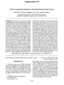
The levelling data (Fig. 2) used is the ANLN (provided by Geoscience Australia [GA]; G. Johnston 2007, pers. comm.), which has received some updates since 1971. The ANLN comprises ∆H from six different levelling orders (see Table 1 in Section 4.2.2 for the number of observations in each). Third-order levelling (maximum allowable √ misclosure of 12 d mm, where d is the distance in km between benchmarks along the levelling route) is the dominant levelling standard in the ANLN (Roelse et al. 1971; Filmer and Featherstone 2009). σi0 for the different levelling types were based on the estimates derived empirically from 1366 ANLN loop closures in Filmer and Featherstone (2009). These unit σi0 were √ propagated along each levelling section as σi0 d. The estimated σi0 from Filmer and Featherstone (2009; FFσi0 in Table 2) were increased slightly (σi0 in Table 2) to allow for the likelihood of compensating errors in the ANLN that would make the empirical estimates over-optimistic and not properly reflect the quality of the levelling (cf. Section 4.2.2). An iterative outlier detection process (Fig. 1) was undertaken (e.g., Schwarz and Kok 1993) on the ANLN using repeated minimal constraints LSA (fixed at one mainland tide gauge and one Tasmanian tide gauge) to identify and re-weight levelling blunders that remain in the ANLN (re-observation was not possible). A significance level of α = 0.001 was used, so that the critical value (CV) for the w -test is ±3.29 (wj = vˆj /σvˆj ; Teunissen 2006b, p. 134). Rather than using an established method of re-weighting outliers (e.g., the Danish method) we determined the re-weighting based on adjacent ANLN loop misclosures, and the minimal detectable bias (MDB; see Teunissen 2006a, p. 67) for each observation using power level γP = 0.80. This was because
17 120°0’E
130°0’E
140°0’E
150°0’E
!!! ! !! !
"
10°0’S
"
! ! !! ! ! ! ! ! ! ! ! ! ! ! ! ! ! ! ! ! !
10°0’S
"
!! !!
!! ! ! ! ! ! ! !!!!! ! ! ! ! !! ! !!! !!! !! ! ! ! ! !! ! ! ! ! ! !!! !!!! ! !!! ! !!!! !!!! ! ! ! ! ! ! !!! ! ! ! !!! ! ! ! ! !!!! !! ! ! !!! ! ! ! ! ! !! ! !! ! ! ! ! ! ! !!! !!! !! ! ! !!!! ! !!! ! ! ! ! ! !! !!!!!! !! ! !! ! !! !!!! ! ! ! !! !! ! !!!!! !! ! ! ! !! ! ! ! !! ! !!! ! ! ! ! ! ! ! ! ! ! ! !!!!!!!! ! ! ! ! ! !! !! ! ! ! !! ! ! ! ! !! !!!!!! !! ! ! ! !!! !!!!! !! ! ! ! !! ! ! ! ! ! ! ! ! ! ! ! !! ! ! ! ! ! ! ! ! ! ! ! ! ! !!! ! ! ! !! ! ! ! ! ! ! ! ! ! ! !! ! ! ! ! ! ! ! ! ! ! ! ! ! !!! !! ! ! ! !! !! !! ! ! ! ! ! !! ! ! ! ! !! ! ! ! ! ! ! !! ! !! !! ! ! ! ! !! ! !!!!! !!!! !!! ! ! !!! ! !! ! !! ! !!!! !!!!!! ! ! ! ! ! ! ! !! ! ! ! ! ! ! ! ! ! ! ! ! ! !! ! !!!!!! ! ! ! !! ! ! ! ! ! !! ! ! ! ! ! ! ! ! ! ! !!! ! ! ! !! !! ! ! ! !! ! !! !! ! ! ! !! ! ! ! ! ! ! ! ! ! ! ! ! ! ! ! ! ! !!!!!! ! !! ! ! ! ! !! !! ! ! !! ! ! ! ! ! ! !! ! ! !! ! ! ! !!!! ! ! ! ! ! ! !! ! ! !! !! ! !! ! !! ! !!! ! !! ! ! ! ! !! !! ! ! ! ! !! ! ! ! ! ! !!! !! !! !!!!! !!!! ! ! ! !! ! ! !! ! !! ! !!! !!! !! ! !!!!! ! ! ! !! !! !! !!! ! ! ! ! ! ! ! ! !! ! ! !! ! ! ! ! !!! !!!!! !!!!!!!!!!!!!!!! ! ! ! ! !!!!! ! ! !! ! ! ! ! ! ! ! ! !! ! ! !!!!!!!!!!!!!!!!!! !! ! ! !!! !!!!! ! ! !! !!!!!! ! !! ! ! ! !! !!!! ! ! ! ! ! ! ! ! ! ! ! ! ! ! ! !! ! ! ! ! ! !! ! ! !! !! ! ! ! ! !!!!!! ! ! ! ! ! !!!!! ! ! ! ! ! ! ! !! !!! ! ! !!! !!!!!!!!!!! ! ! ! ! !!!! ! ! ! !! ! ! ! !!!!!!!!! !! ! !! ! !! !! ! ! ! ! ! ! ! ! ! !! ! ! ! ! ! ! !!! ! ! !! ! ! ! ! !! ! !! !! ! ! ! ! ! ! !! !!!!!! ! ! ! ! ! ! !! !! ! ! !!! ! !!!! ! ! ! ! !! ! ! ! ! ! ! ! ! ! ! ! ! ! !! ! ! ! ! ! ! ! ! ! ! ! ! ! ! ! ! ! ! ! ! ! ! ! ! ! ! ! !!!!!! ! ! ! ! ! ! ! ! !! ! ! ! ! ! ! ! !! ! !! ! ! !! ! ! ! ! ! ! ! ! ! ! ! !!!!! ! !! ! ! ! ! ! ! ! ! ! ! ! ! ! ! ! !! ! !!! !! ! ! ! !! ! ! ! !! ! ! ! ! ! ! !! !!! ! ! ! ! ! ! ! ! ! !! !!! ! !! ! ! ! ! ! ! !! ! ! ! ! ! ! ! ! ! ! ! ! ! ! ! ! ! ! ! ! ! ! ! ! ! ! ! ! ! ! ! ! ! ! ! ! ! ! ! ! !! ! ! !! !!! ! ! !!!! ! !!! ! !! !! ! ! ! ! ! ! ! ! ! ! ! !!!!!! ! !! !! !! !! ! ! ! !! ! ! ! ! ! ! ! ! !!! !! ! ! ! ! ! ! ! ! ! ! ! ! !!!!!!!!! ! !! !! !! ! !! ! ! ! ! !! ! ! !! !! ! ! ! ! ! !! ! ! ! ! ! ! ! ! ! ! ! ! ! !!! ! ! ! ! ! !!! ! ! ! ! ! ! ! ! ! !!!! !!!!!!!!!! ! !! ! !!!!! ! ! ! !!! !! ! ! !! ! !!! ! ! ! !!! ! ! ! ! !! ! ! ! !! ! !! ! ! !!! ! ! ! ! ! !! !!! ! !! ! !! ! ! ! ! !!! !! !!!!! ! !!! ! ! ! ! ! !!!!!!! ! ! ! !!! ! ! !!! ! !! !!!! !! !!!! ! ! ! !! ! ! ! ! ! ! ! !!! ! ! ! ! !! ! ! !! ! ! !! !! !!!!!! ! ! ! ! !!! ! ! ! ! ! ! !! ! ! ! ! ! !!! ! !!!! ! ! !! ! ! ! ! ! !! ! !!!!! !! !! ! ! !!! ! ! !! ! !!!! ! !! ! ! ! !!!! ! !! ! ! ! !! !! ! ! !! ! ! !! ! ! ! !!! ! ! ! ! !!!! !! ! ! !!!!!!! ! !! ! !! !!! ! ! !!! ! ! !! ! !! ! !! !! ! ! ! !! ! ! !! !! ! ! ! ! ! ! ! ! ! ! ! ! ! ! ! ! ! ! ! ! ! !! ! ! ! ! !! ! ! ! ! ! ! ! ! ! ! ! ! ! ! ! ! !!!! ! ! ! ! ! ! ! ! ! ! !!! ! ! ! ! ! ! ! ! ! ! ! ! ! ! ! ! ! !!!!!!!!!! ! ! ! ! !! ! ! ! ! ! ! !! ! !!! ! ! !! !!!!!!!! ! ! ! ! ! ! ! !! ! ! ! ! ! ! !! !! !!!! ! !! ! ! ! ! ! ! !!! ! ! ! !!!!! ! !! ! ! ! !! !! !! ! ! ! ! ! !!!!!!!!! ! ! ! ! ! ! ! ! ! ! ! ! ! ! ! ! ! ! ! ! ! ! ! ! !! ! ! ! ! ! !!! ! ! ! ! ! ! ! !!!! ! ! ! ! ! !! ! ! !! ! !! ! ! ! ! ! ! ! ! ! ! ! ! ! ! ! ! ! ! ! !! ! ! ! ! !! ! !!! ! !!!!! !!!!! ! !!!! ! ! !! !! ! !!!!! ! !!! ! !!!!!!!!! ! ! ! ! ! ! ! ! ! !! ! ! ! ! ! ! ! ! ! ! ! ! ! !! !! ! ! ! ! ! ! ! ! ! !! ! ! ! ! ! ! !!! !! ! !! !! ! ! ! ! !!! ! ! ! ! ! ! ! ! ! ! ! ! !! ! !! ! ! ! ! ! ! ! ! ! ! ! ! ! ! ! !!!! ! ! !!!! ! ! ! !!!!!!! ! ! ! ! ! ! !!!!! ! !! ! ! ! !!! ! ! ! ! ! ! ! ! ! ! ! ! ! ! ! ! ! ! ! ! ! ! ! ! ! ! ! ! ! ! ! ! ! ! ! ! ! ! ! ! ! ! ! ! ! ! ! ! ! ! ! ! ! ! ! ! ! ! ! ! ! ! ! ! ! ! ! ! ! ! ! ! ! ! !!! ! ! !!!!!! !! ! ! !!!!!!! !! !!!! ! ! ! !!!!!! ! ! !!! ! ! ! ! ! ! ! ! ! ! ! ! ! ! !! ! !! ! ! ! ! ! ! ! ! ! ! ! ! !!!!!!! ! !!!! ! ! ! ! !! ! ! !!!!!!!!!! ! !!!!!! ! ! ! ! ! ! ! !! ! ! !! ! ! ! ! !! ! ! ! ! ! ! ! !! ! ! ! ! ! ! ! ! ! ! ! !!! ! !! !! ! ! ! ! !! ! ! ! ! ! !! ! ! ! ! !! !! !!! ! ! ! ! ! ! ! ! ! ! ! ! ! !!!! !! ! ! !! ! ! ! ! ! !!! ! ! ! ! !!! ! ! ! ! ! ! ! !! ! ! ! ! ! ! ! ! ! ! ! ! ! ! ! ! ! ! ! ! ! ! ! ! ! ! ! ! ! ! ! ! ! ! ! ! ! ! ! ! ! ! ! ! ! ! ! ! ! ! ! ! ! ! ! ! ! ! ! ! ! ! ! ! ! ! ! ! ! ! !! ! ! ! ! ! ! ! ! ! ! !! !!! ! ! ! !! !! ! ! ! ! ! ! ! ! ! ! ! ! ! ! ! ! ! ! ! ! ! ! ! ! ! ! ! ! ! !!!! ! ! ! ! ! ! ! ! ! ! ! ! !! !!! !!! ! ! ! ! ! !!! ! !! ! ! ! ! ! ! ! ! ! ! ! ! ! !! ! !!! ! ! !! ! ! ! ! ! ! ! ! ! ! !! ! ! ! !! ! ! ! ! ! ! ! ! !! ! ! ! ! !! ! ! ! ! ! ! ! ! ! ! ! ! ! ! ! ! ! ! ! ! ! ! ! ! ! ! ! ! ! ! !! !! ! ! ! ! !!! ! ! ! ! ! ! ! ! ! ! !!!! ! ! ! ! ! ! ! ! ! ! ! ! ! ! ! ! !! ! ! ! !! ! ! ! ! ! ! ! ! ! ! ! ! ! ! ! ! ! ! ! ! ! !!!! ! !! ! !! !!!! ! ! ! ! ! ! !! ! ! ! ! ! !! ! ! ! ! ! ! ! ! ! !!!!! !! !! ! ! ! !! ! ! ! ! ! ! ! ! ! ! ! ! ! ! ! ! ! ! ! ! ! ! ! ! ! ! ! ! ! ! ! ! ! ! ! ! ! !! ! !! ! !! ! ! ! ! ! ! ! ! ! !! ! ! ! ! ! ! ! ! ! ! ! ! ! ! ! ! ! ! ! ! ! ! ! ! ! ! ! ! ! ! ! ! ! ! ! ! ! ! ! ! ! ! ! ! !! !! !! ! ! ! ! ! ! ! ! ! ! ! ! ! ! ! ! ! ! ! ! ! !!!!!!!! ! ! ! !! ! !!! ! ! !! ! ! ! ! !!!!!!! !!! ! ! !!!! ! ! ! !!!!!!!!!! !!! ! ! ! ! ! ! ! ! !!! ! ! ! ! !! ! ! ! ! ! !! ! ! ! ! ! ! ! ! ! !! ! !!!! !!! ! ! ! ! ! ! ! ! ! ! ! !!!!!! !!! ! !!!! ! ! ! ! ! !! ! !!! ! ! ! ! ! ! ! ! ! ! ! ! ! ! ! ! ! !! !!! !! ! ! ! ! ! ! !!! ! ! !! ! ! !! !! ! ! ! ! ! ! !! ! ! !!! ! ! ! ! ! ! ! ! ! !!! ! !! !! !!! ! ! ! ! ! ! ! ! ! !!! ! ! ! ! !!!!!!! ! ! ! ! ! ! ! ! ! ! !!! ! ! ! ! ! ! ! !! ! !! !! ! ! ! ! ! ! ! ! ! ! !!! !! !! ! ! !! ! !!!!!! ! !! ! ! ! ! ! !! ! ! !! !!!! !! ! !! ! ! ! ! !!!! ! !! !!! ! ! ! !! !!! ! !! ! ! ! ! !!!!! ! !! ! ! ! ! ! ! !!! ! ! ! ! !! !! ! ! !! ! ! ! ! ! ! ! ! !! !!!! ! ! ! ! ! ! !! !! ! ! ! !!!!!! ! ! !! ! ! !! ! !! ! !! ! ! ! ! ! ! ! ! !! ! ! ! !! ! !!!!! !! ! ! ! !! !! ! ! ! ! ! ! ! ! ! ! ! ! ! ! ! ! ! ! ! ! ! ! ! ! ! ! ! ! ! ! ! ! ! ! ! ! ! ! ! ! ! ! ! ! ! ! ! ! ! ! ! ! ! ! ! ! ! ! ! !! ! !! ! ! ! ! !!!!!! ! ! ! !!! ! ! ! !! ! ! ! ! ! ! ! ! ! !! ! ! !! ! ! !!! ! ! ! !! ! ! ! ! ! ! ! ! ! ! !! !!! ! !! ! ! !! ! !! !! ! !! ! !! !! ! ! ! ! !!!! !!!!! ! ! ! ! !!!! !! ! ! ! ! ! ! ! ! ! !! ! ! ! !! !!! ! ! ! ! ! ! ! ! ! !!!! ! ! ! ! ! ! ! !! ! ! ! ! !! ! ! ! ! ! ! ! ! ! ! ! ! ! ! ! ! ! !!!! ! !! ! ! !! ! ! !! ! ! !! !!!! ! !!! ! ! ! ! ! !!! ! ! !!! ! ! !!! ! ! ! ! ! ! ! ! !!!!!!! !!!!!! ! ! ! !! ! !! ! !!! !!! ! ! ! !! !!!! !! ! ! ! ! ! ! !! !! ! !! ! !! ! ! ! ! !! ! !! ! !! ! ! ! ! ! ! ! ! ! ! ! ! !! ! ! ! !! ! ! ! !!!!!! ! !! ! ! ! ! !!!! ! ! ! ! !! ! ! ! ! ! ! ! ! ! ! ! ! ! ! ! ! ! ! ! ! ! !! ! ! ! ! ! !!!! ! ! ! ! !! ! ! ! !! ! !!! !! ! ! ! ! ! ! !!!! !! ! ! ! ! ! ! ! ! ! !!!! ! ! ! !!! ! ! ! ! ! !! !!!!!! ! ! ! !!! ! ! !! ! ! ! ! ! ! ! ! ! ! ! ! ! ! ! ! ! ! ! ! ! ! ! ! ! ! ! ! ! ! ! ! ! ! ! ! ! ! ! ! ! ! ! ! ! !! ! !! ! ! ! !! !!! ! ! ! ! !! ! ! ! ! ! ! !!!!! ! ! ! ! ! ! !! ! ! ! ! ! !! ! !!!! ! !!! !! !!!!!!!! !!!!!!!!! ! !!!!!!!!!!!!!!!!!!! ! ! !!!!! !! !!!!! ! !! !! ! !!! ! !! ! !!!! ! ! !! ! ! !!!!!!! ! !!! ! ! ! ! ! ! ! !!! !! !!!! ! ! ! !! ! !! ! ! ! ! ! ! ! ! ! ! ! ! ! ! ! ! ! !! ! ! ! ! ! ! ! ! ! ! ! ! ! ! ! ! ! !! ! ! !!! ! ! !!!! ! ! ! ! !! ! ! !!!! ! !! ! ! ! ! ! ! !! ! ! ! ! ! ! ! ! ! !!!!!! ! ! ! ! ! ! ! ! ! !! !! !! !!!! !! ! ! ! !!!! !!! ! ! ! ! ! ! !!! ! ! !! ! !! ! ! ! !!!!!! ! ! ! ! ! ! ! ! ! ! ! ! ! ! ! ! !! ! ! ! ! ! ! ! ! ! ! ! ! ! ! ! ! ! ! ! ! ! ! ! ! ! ! ! !!!!! ! ! !!!!! !! ! ! ! ! ! ! !!! ! !! ! ! ! ! ! !! !!!!!!!!!!!! ! ! ! ! !!!!!!!! !! !! ! ! ! ! ! ! ! !!!!!!!!!!!! ! !! ! ! ! ! ! ! !!!!!!! !! ! ! ! ! !!!!!!! ! !! ! ! ! !! !!!!! ! ! ! ! ! ! ! ! ! ! ! ! ! !! ! !! ! !!! !! ! ! !! ! ! ! ! ! ! ! ! !!!! ! ! ! ! ! ! ! ! ! ! ! ! ! ! ! ! ! ! !! ! ! ! ! ! ! ! ! ! ! ! ! ! ! ! ! ! ! ! ! ! ! ! ! ! ! ! ! ! ! ! ! ! ! ! ! ! ! ! ! ! ! ! ! ! ! !! ! ! ! ! ! ! ! ! ! ! ! ! ! ! ! ! ! ! ! ! ! ! ! ! ! ! ! !! ! ! ! ! ! ! ! ! !! ! !! ! ! ! !! ! ! ! ! ! ! ! ! ! ! ! ! ! ! ! ! ! ! ! ! ! ! ! ! ! ! ! ! ! ! ! ! !!! ! ! ! ! ! ! !! ! ! ! ! ! ! ! ! ! ! ! ! ! ! ! ! ! ! ! ! ! ! ! ! ! ! ! ! ! ! ! ! ! ! ! ! ! ! ! ! ! !! ! ! ! ! !! !! ! ! ! ! ! ! !! ! ! ! ! ! !! ! ! ! ! ! ! ! ! ! ! ! ! !! ! ! ! ! ! ! ! ! ! ! ! ! ! ! ! ! ! ! ! ! ! ! ! ! ! ! ! ! ! ! ! ! ! ! ! ! !! ! ! ! ! ! ! ! ! ! ! ! !! ! ! ! ! ! !! ! ! ! ! ! ! !! ! ! ! ! ! ! ! ! ! ! ! ! ! ! ! ! ! ! ! ! ! ! ! ! ! ! ! ! ! ! ! ! ! ! ! ! ! ! ! ! ! ! ! ! ! ! ! ! ! ! ! ! ! ! ! ! ! ! ! ! ! ! ! ! ! ! !! ! !! ! ! ! ! ! ! ! ! ! ! ! ! ! ! ! ! ! ! !! ! ! ! ! ! ! ! ! ! ! ! ! ! ! ! ! ! ! ! ! ! ! ! ! ! ! ! ! ! ! !! ! ! ! ! ! ! ! ! ! ! ! ! ! !! ! ! ! ! ! ! ! ! ! ! ! ! !! ! ! !!!! ! ! ! ! ! ! !! ! !! ! ! ! ! ! ! ! ! ! ! ! ! ! ! ! ! ! ! ! ! ! ! ! ! ! ! ! ! ! !! ! ! ! ! ! ! ! ! ! ! ! ! ! ! ! ! ! ! ! ! ! ! ! ! ! ! ! ! ! ! ! ! ! ! ! ! ! ! ! ! ! ! ! ! ! ! ! ! ! ! ! ! ! ! ! ! ! ! ! ! ! ! ! ! ! ! ! ! ! ! ! ! ! ! ! ! ! ! ! ! ! ! ! ! ! ! ! ! ! !! ! ! ! ! ! ! ! ! ! ! ! ! ! ! ! ! ! ! ! ! ! ! ! ! ! ! ! ! ! ! ! ! ! ! ! ! ! ! ! ! ! ! ! ! ! ! ! ! ! ! ! ! ! ! ! ! ! ! ! ! ! ! ! ! ! ! ! ! ! ! ! ! ! ! ! ! ! ! ! ! ! ! !! ! ! ! ! ! ! ! ! ! ! ! ! ! ! ! !! ! ! ! ! ! ! ! ! ! ! ! ! ! ! !! ! ! ! ! ! ! ! ! ! ! ! ! ! ! !! ! ! ! ! ! ! ! ! ! ! ! ! ! ! ! ! ! ! ! ! ! ! ! ! !! ! ! ! !! ! ! ! ! ! ! ! ! ! ! ! ! ! ! ! ! ! ! ! ! ! !! ! ! ! ! ! ! ! ! ! ! ! ! ! ! ! ! ! ! ! !! ! !! ! ! ! ! ! ! ! ! ! ! ! ! ! ! ! ! ! ! ! ! !! ! ! ! ! ! ! ! ! ! ! ! ! ! ! ! ! ! ! ! ! ! ! ! ! ! ! ! ! ! ! ! ! ! ! ! ! ! ! ! ! ! ! ! ! ! ! !! ! ! ! ! ! ! ! ! ! ! ! ! ! ! ! !! ! ! ! ! ! ! ! ! ! ! ! ! ! ! ! ! ! ! ! ! ! ! ! ! ! ! ! ! ! ! ! ! ! ! ! ! ! ! ! ! !!! ! ! ! !! ! ! ! ! ! ! ! ! ! ! ! ! ! ! ! ! ! ! ! ! ! ! ! ! ! ! ! ! ! ! ! ! ! ! ! ! ! ! ! ! ! ! ! ! ! ! ! ! ! ! ! ! ! ! ! ! ! ! ! ! ! ! !! ! ! ! ! ! ! ! ! ! ! !! ! ! !! ! ! ! ! ! ! ! ! ! ! ! ! ! ! ! ! ! ! ! ! ! ! ! ! ! ! ! !! ! ! ! ! ! ! ! ! ! ! ! ! ! ! ! ! ! ! ! ! !! ! ! ! ! ! ! ! ! ! ! ! ! ! ! ! ! ! ! ! ! ! ! ! ! ! !! ! ! ! ! ! ! ! ! ! ! ! ! ! ! ! ! ! ! ! ! ! ! ! ! ! ! ! ! !! ! ! ! ! ! ! ! ! ! ! ! ! ! ! ! ! ! ! ! ! ! ! ! ! ! ! !!! ! !! ! ! ! ! ! ! ! ! ! !!!!!! ! ! ! ! ! ! !!!! !! ! ! ! ! ! ! ! ! ! ! ! ! ! ! ! ! ! ! ! ! ! ! ! ! ! ! ! ! ! ! ! ! ! ! ! ! ! ! ! ! !! ! ! ! ! ! ! ! ! ! ! ! ! ! ! ! ! ! ! ! ! ! ! ! ! ! ! ! ! ! ! ! ! ! ! ! ! ! ! ! ! ! ! ! ! ! ! ! ! ! ! !! ! ! ! ! ! ! ! ! ! ! ! ! ! ! ! ! ! ! !! ! ! ! ! ! ! ! ! ! ! ! ! ! ! ! ! ! ! ! ! ! ! ! ! ! ! ! ! ! ! ! ! !! ! ! ! ! ! ! ! ! ! ! ! ! ! ! ! ! ! ! ! ! ! ! ! ! ! ! ! ! !!!! ! ! ! ! ! ! ! ! ! ! ! ! ! ! ! ! ! ! ! ! ! ! ! ! ! ! ! ! ! ! ! ! ! ! ! ! ! ! ! ! !! ! ! ! ! ! ! ! ! ! ! ! ! ! ! ! ! ! ! ! ! ! ! ! ! ! ! ! ! ! ! ! ! ! ! ! ! ! ! ! ! ! ! ! ! ! ! ! ! ! ! ! ! ! ! ! ! ! ! ! ! ! ! ! ! ! ! ! ! ! ! ! ! ! ! !!!! ! ! ! ! ! ! ! !! ! ! ! ! ! ! ! ! ! !!!! ! ! ! ! ! ! ! ! ! ! ! ! ! ! ! ! ! ! ! ! ! ! ! ! ! ! ! ! ! ! ! ! ! ! ! ! ! ! ! ! ! ! ! ! ! ! ! ! ! ! ! ! ! ! ! ! ! ! ! ! ! ! ! ! ! ! ! ! ! ! ! ! !! ! ! ! ! !! ! ! ! !! ! ! ! ! ! ! ! ! ! ! ! ! ! ! ! ! ! ! ! ! !! ! ! ! ! ! ! ! ! ! ! ! ! ! ! ! ! ! ! ! ! ! ! ! ! !! ! ! ! ! ! ! ! ! ! ! ! ! ! ! ! ! ! ! ! ! ! ! ! !! ! ! ! ! ! ! ! !! ! ! ! ! ! ! ! ! ! ! ! ! ! ! ! ! ! ! ! ! ! !! ! ! ! ! ! ! ! ! ! ! !! ! ! ! ! ! ! ! ! ! ! ! ! ! ! ! ! ! ! ! ! ! ! ! ! ! ! ! ! ! ! ! ! ! ! ! ! ! ! ! ! ! ! ! ! !! ! ! ! ! ! ! ! ! ! ! ! ! ! ! ! ! ! ! ! ! ! ! ! ! ! ! ! ! ! ! ! ! ! ! ! ! ! ! ! ! ! ! ! ! ! ! ! ! !! ! ! ! ! ! ! ! ! ! ! ! ! ! ! ! ! ! ! ! ! ! ! ! ! ! ! ! ! ! ! ! ! ! ! ! ! ! ! ! ! ! ! ! ! ! ! ! ! ! ! ! ! ! ! ! ! ! ! ! ! ! ! ! ! ! ! ! ! ! ! ! ! ! ! ! ! ! ! ! ! ! ! ! ! ! ! !!! ! ! ! ! ! ! ! ! ! ! !!! ! ! ! ! ! ! ! ! !! ! ! ! ! ! ! ! ! ! ! ! ! ! ! ! ! ! ! ! ! ! ! ! ! ! ! ! ! ! ! ! ! ! ! ! ! ! ! ! ! !! ! ! ! ! ! ! ! ! ! ! ! ! ! ! ! ! ! ! ! ! ! ! ! ! ! ! ! ! ! ! ! ! ! ! ! ! ! ! ! ! ! ! ! ! ! ! ! !! ! ! ! ! ! ! ! ! ! ! ! ! ! ! ! ! ! ! ! ! ! ! ! ! ! ! ! ! ! ! ! ! ! ! ! ! ! ! !!! ! ! ! ! ! ! ! ! ! ! ! ! ! ! ! ! ! ! ! ! ! ! ! ! ! ! ! ! ! ! ! ! ! ! ! ! ! ! ! ! ! ! ! ! ! ! ! ! ! ! ! ! ! ! ! ! ! ! ! ! ! ! ! ! ! ! ! ! ! ! ! ! ! ! ! ! ! ! ! ! ! ! ! ! ! ! ! ! ! ! ! ! ! ! ! ! ! ! ! ! ! ! ! ! ! ! ! ! ! ! ! ! ! ! ! ! ! ! ! ! ! ! ! ! ! ! ! ! !! ! ! ! ! !! ! ! ! ! ! ! ! ! ! ! ! ! ! ! ! ! ! ! ! ! ! ! ! ! ! ! ! ! ! ! ! ! ! ! ! ! ! ! ! ! ! ! ! ! ! ! ! ! ! ! ! ! ! ! ! ! ! ! ! ! ! ! ! ! ! ! ! ! ! ! ! ! ! ! ! ! ! ! !! ! ! ! ! ! ! ! ! ! ! ! ! ! ! ! ! ! ! ! ! ! ! ! ! ! ! ! ! ! ! ! ! ! !! ! ! ! ! ! ! ! ! ! ! ! ! ! ! ! ! ! ! ! ! ! ! ! ! ! ! ! ! ! ! ! ! ! ! ! ! ! ! ! !! ! !! ! ! ! ! ! ! ! ! !! ! ! ! ! ! ! ! ! ! ! ! ! ! ! !! ! ! ! ! ! ! ! ! ! ! ! ! !! ! ! ! !! ! ! ! ! ! ! ! ! ! ! ! ! ! ! ! ! ! ! ! ! ! ! ! ! ! ! ! ! ! ! ! ! ! ! !! ! ! ! ! ! ! ! ! ! ! ! ! ! ! ! ! ! ! ! ! ! ! ! ! ! ! ! ! ! ! ! ! ! ! ! ! ! ! ! ! ! ! ! ! ! ! ! ! ! ! ! ! !! ! ! !! ! ! ! ! ! ! ! ! ! ! ! ! !! ! ! ! ! ! ! ! ! ! ! !! ! !! ! ! ! ! ! ! ! ! ! ! ! ! ! ! ! ! ! ! ! ! ! ! ! ! ! ! ! ! ! ! ! ! ! ! ! ! ! ! ! ! ! ! ! ! ! ! ! ! ! ! ! ! ! ! ! ! ! ! ! ! ! ! ! ! ! ! ! ! ! ! ! ! !! ! ! ! ! ! ! ! ! ! ! ! ! ! ! ! ! ! ! ! ! ! ! ! ! ! ! ! ! ! ! ! ! !! ! ! ! ! ! ! ! ! ! ! ! ! ! ! ! ! ! ! ! ! ! ! ! ! ! ! ! ! ! ! ! ! ! ! ! ! ! ! ! ! !! ! ! ! ! ! ! ! ! ! ! ! ! ! ! ! ! ! ! !! ! ! ! ! ! ! ! ! ! ! ! ! ! ! ! ! ! ! ! ! ! ! ! ! ! ! ! ! ! ! ! ! ! ! ! ! ! ! ! ! ! ! ! ! ! ! ! ! ! ! ! ! ! ! ! ! ! ! ! ! ! ! ! ! ! ! ! ! ! ! ! ! ! ! ! ! ! ! ! ! ! ! ! ! ! ! ! ! ! ! ! ! ! ! ! ! ! ! ! ! ! ! ! ! ! ! ! ! ! ! ! ! ! ! ! ! ! ! ! ! ! ! ! ! ! ! ! ! ! ! ! ! ! ! ! ! ! ! ! ! ! ! ! ! ! ! ! ! ! ! ! ! ! ! ! ! ! ! ! ! ! ! ! ! ! !! ! ! ! ! ! ! ! ! ! ! ! ! ! ! ! ! ! ! ! ! ! ! ! ! ! ! ! ! ! ! ! ! ! ! ! ! ! ! ! ! ! ! ! ! ! ! ! ! ! ! ! ! ! ! ! ! ! ! ! ! ! ! ! ! ! ! ! ! ! ! ! ! ! !! ! ! ! ! ! ! ! ! ! ! !! ! ! ! ! ! ! ! ! ! ! ! ! ! ! ! ! ! ! ! ! ! ! ! ! ! ! ! ! ! ! ! ! ! ! ! ! ! ! ! !! !! ! !! ! ! ! ! ! ! ! ! ! ! ! ! ! ! ! ! ! ! ! ! ! ! ! ! ! ! ! ! ! ! ! ! ! ! ! ! ! ! ! ! ! ! ! ! ! ! ! ! ! ! ! ! ! ! ! ! ! !! ! ! ! ! ! ! ! ! ! ! ! ! ! ! ! ! !! ! ! ! ! ! ! ! ! ! ! ! ! ! ! ! ! ! ! ! ! ! ! !! !! ! ! ! !! ! ! ! ! ! ! ! ! ! ! ! ! ! ! ! ! ! ! ! ! ! ! ! ! ! ! ! ! ! ! ! ! !!! ! ! !!!!! ! ! ! ! ! !! ! ! ! ! ! ! ! ! ! ! ! ! ! ! ! ! ! ! ! ! ! ! ! ! ! ! ! ! ! ! ! ! ! ! ! ! ! ! ! ! ! ! ! ! ! ! ! ! ! ! ! ! ! ! ! ! ! ! ! ! ! ! ! ! ! ! ! ! ! ! ! ! ! ! !
!
!
!
"!!!
!
"
! !
"
! ! ! ! ! !! ! !
!
!
!
! !
!
! !
!
!
!
! !
!
!
!
! !
!
! !!
! ! ! !
!
!
" "!!!
! !
! !
!
!
!
!
! ! !
!
!
!
"
"
!
!
!
!
!
"
! ! ! !! ! ! ! ! ! ! ! !
"!
!
! ! ! !! ! ! ! ! ! ! ! ! ! ! ! ! ! ! ! !! !! ! ! !! !! ! ! ! !! !! ! ! ! !! ! ! ! ! ! !! !! ! ! !! ! ! ! ! ! ! ! ! ! ! !!! ! ! ! !! ! !! ! ! ! !! ! ! ! ! ! ! ! !
"
"
!
!
"
"
!!
!
!
!
!
! ! ! !!!
! !
!
!
!
!
" "
!
"!
! ! !
!
!
!
!
!
" 30°0’S
!
!
!
! ! ! ! !! !
!
!
!
"
!!
!
!
! ! !
20°0’S
!
!
"
!
!
!
!
!! !! !
!
!
!
!!
!!
! ! ! ! !! ! !! ! ! ! ! ! ! ! !! ! ! ! ! ! ! ! ! ! !! ! ! ! !! !! !
!
20°0’S
"
"
!!
"
30°0’S
!!
" "
"" " ! !
0
40°0’S
250
500
1,000 Kilometers
"
! ! ! ! ! ! ! ! ! ! ! ! ! ! ! ! ! ! ! !
! !!!
! ! ! ! ! ! ! !
40°0’S
"
110°0’E
120°0’E
130°0’E
140°0’E
150°0’E
160°0’E
Fig. 2 The Australian national levelling network (ANLN). First order sections are in orange, second order in green, third order in grey, fourth order in purple, one-way (third order) in red and two-way (order undefined) in blue. The 32 tide-gauges used to fix the AHD and also to constrain the CLSA for this study are shown as black squares. The 277 GPS points used are black circles. Lambert projection, ANLN, GPS and tide gauge data courtesy of Geoscience Australia.
the low redundancy and suspected multiple outliers in some remote parts of the ANLN required manual assessment to reduce the risk that a ‘good’ observation (not containing an error) could be incorrectly re-weighted (type I error), or one (or more) observations that may contain errors could be accepted as correct (type II error). The process was iterated until |wj | < |CV| ∀ ∆H N . We assume for the purpose of this study that all blunders were appropriately re-weighted.
18
130˚
120˚
140˚
150˚
−10˚
−10˚
−20˚
−20˚
−30˚
−30˚
−40˚
−40˚ 120˚
130˚
140˚
150˚
Fig. 3 The 277 GPS points used to constrain the CLSA are red circles (cf. Fig. 2) and the 765 GPS points not used are black circles. All red and black circles comprise the 1042 GPS points used to estimate the CARS2009-ITRF2000 offset. Lambert projection, GPS data courtesy of Geoscience Australia.
The 10 × 10 AGQG09 quasigeoid model (Featherstone et al. 2011) is used for this study, with the AGQG09 height anomaly (ζ) bicubically interpolated at the φ and λ of each GPS h. AGQG09 is the gravimetric component of AUSGeoid09 (Featherstone et al. 2011). A set of 1,052 3D GPS coordinates were supplied to us by GA (N. Brown 2009, pers. comm.), processed in the International Terrestrial Reference Frame 2005 (ITRF2005; Altamimi et al. 2007) at epoch 2000 (Hu 2009). Ten GPS points were removed with apparent errors of up to 1.5 m which were assumed to be antenna height blunders. Of the 1,042 GPS points (Fig. 3), 765 were not used as constraints in the CLSA, because many were redundant observations connected to the same benchmark, and some were observed tens of kms from the nearest levelling JP to which they were connected. We selected 277 GPS points as CLSA constraints (Fig. 2 and Fig. 3), which
19
provided a reasonably even distribution across the ANLN, but also constraining specific parts of the ANLN based on information from the outlier detection process. The GPS-derived h were provided with their associated SD (σh ) from the internally propagated precision of the Bernese processing. The average σh for the entire set after scaling the internal precision by 10 (e.g., Rothacher 2002) is ±26 mm (N. Brown 2009, pers. comm.), which was adopted as σh for all GPS points. The full variancecovariance matrix from the Bernese processing was not available. An approximate a priori SD estimate of ±100 mm is made for the combined h − ζ constraint (σhζ ) (cf. Featherstone et al. 2011). The MSL observations used are the 32 (mostly) three-year tide gauge observations used in the realisation of the AHD (Fig. 2; Roelse et al. 1971), primarily because of availability, as many tide gauges with longer observation periods are not directly connected by levelling to the ANLN. These 32 AHD tide gauge records were used by Featherstone and Filmer (2012) to demonstrate that a combination of MSL-MDT, h−ζ at tide gauges and the ANLN removed the north-south tilt in the AHD, suggesting that they are a reasonable representation of (relative) MSL around Australia. The MDT model used is the oceanographic-only MDT computed from the digital climatology, CSIRO Atlas of Regional Seas 2009 (CARS2009; Ridgway et al. 2002; Dunn and Ridgway 2002), which is available at http://www.marine.csiro.au/ dunn/cars 2009/. Featherstone and Filmer (2012) demonstrated that the oceanographic-only MDT model CARS2009 performed better in coastal regions than geodetic-only MDTs (satellite altimetry-derived mean sea surface (MSS) minus a geoid model) and combined MDT models (combination of geodetic and oceanographic MDTs). An approximate a priori SD for combined MSL-MDT observations at 32 tide gauges (σT G ) is ±50 mm. This is estimated to comprise ±20 mm for σM SL and ∼ ±45 mm
20
for σM DT (cf. Filmer 2014) on the assumption that no correlation exists within QT G0 . There are no formal error estimates for either of these data sets, so therefore no covariance information. We will assume QT G0 to be diagonal for this reason, and also for ease of computation, as is often the case in geodetic applications, although acknowledging the impact that excluding covariance information may have on the computed VCE (e.g., Fotopoulos 2005). A bias of −165±120 mm is calculated between the mean of 1,042 Hhζ and the corresponding H N from a LSA of the ANLN constrained at 32 tide gauges by HT G (CARS2009). We used the full data set (1042 GPS points) to estimate the datum bias because we considered this to be representative of the complete data set. The bias using 277 GPS points selected as CLSA constraints was −171 ± 134 mm, which can be considered the same as for the 1042 GPS points given that the 6 mm difference is much less than the associated precision. The bias is removed from CARS2009 MDT heights so that the zero-reference level for the CLSA is ITRF2005 (epoch 2000) as determined in the processing of h. Vertical datum unification between ANLN(mainland) and ANLN(Tas) is achieved through CARS2009 at 30 AHD tide-gauges on the mainland and two in Tasmania, by removing the CARS2009 MDT offset (Filmer and Featherstone 2012a).
4.2 Results
4.2.1 VCE computation
The CLSA was conducted using the Survey Network Adjustment Program (SNAP), which is freely available at http://www.linz.govt.nz/geodetic/software-downloads. This software allows for the CLSA formulation with the weighted constraints as set out in
21
Section 3.2. The output from this adjustment included the necessary information rj , vˆj , and the input Qy . The SVCE was computed using code written to (1) separate the SNAP output and input data into the separate components; (2) compute σ ˆ i2` ∀ i using Eq. (5); (3) scale each Qi to update Qy ; and (4) iterate this procedure until σ ˆi2` is (or very close to) unity. Due to the diagonal Qy and the simplified solution used, each iteration is computed in a few seconds. The computation of σσ2ˆ 2 using Eqs. (14) to (16) is a much more time consuming i
process because each computation (iteration) requires the repeated multiplication of ∼7,600 × 7,600 matrices and several inversions of similar sized arrays. In Eq. (16), κ is set to zero (Teunissen and Amiri-Simkooei 2008), as it is assumed that our data is normally distributed. We used Crout’s algorithm (Press et al. 1992, p. 33) for lowerupper decomposition for matrix inversion, which was adapted from subroutines in Press et al. (1992, Ch.2.3-2.4). Each computation (one iteration) of Qσˆ 2 took ∼50 hours on a Linux server (256GB RAM, 2.90GHz CPU). This code was modified to compute LS-VCE using Eqs. (9) to (13), which took ∼23 hours per iteration, but this yielded both σ ˆi2 and σσ2ˆ 2 . i
4.2.2 VCE results
The results are arranged in Table 1 to show σ ˆi2 , σσ2ˆ 2 and σσˆ 2 computed using Eq. (6) and Eq. (18) respectively, with σσˆ 2 = i
q
i
i
σσ2ˆ 2 . Table 2 shows σi` representing the SD of i
the different observation types after each VCE iteration, with σσˆiF (F = 7) computed as per Eq. (19), which indicates the contribution of σσ2ˆ 2 to the uncertainty in σi7 . i
Graphical representations of σ ˆi2` and σσˆ 2 in Figs. 4 - 8 show comparisons of the LSi`
VCE and SVCE converging towards unity, and the changes in σσˆ 2 with each iteration. i`
All
σ ˆi2
were positive, but the off diagonal elements in Qσˆ 2 were small and mostly
22 2 and σ Table 1 σ ˆi2 , σσ σ ˆ 2 computed for the SVCE. The number of observations for each ˆ2 i
i
observation group and their percentage of total number of observations (7614) is also shown. 2 and σ σ ˆi2 , σσ σ ˆ 2 are unitless. ˆ2 i
i
σ ˆi2
2 σσ ˆ2
σσˆ 2
no. obs
% of total
First
0.9852
0.0133
±0.1155
941
12.4
Second
1.3590
0.0613
±0.2477
282
3.7
Third
1.2145
0.0023
±0.0474
5630
73.9
Fourth
2.1605
0.4753
±0.6894
51
0.7
One-way
0.9897
0.0129
±0.1135
347
4.6
Two-way
1.0961
0.1155
±0.3399
54
0.7
MSL-MDT
2.7201
0.8319
±0.9121
32
0.4
h−ζ
0.6310
0.0048
±0.0692
277
3.6
i
i
negative, reflecting that no covariance information was used in Qy . The SVCE and LS-VCE σ ˆi2 were the same (cf. Teunissen and Amiri-Simkooei 2008, Section 7), or very close, as shown in Table 2. The highly unbalanced data (Table 1) has resulted in a wide range of uncertainties for σ ˆi2 , indicating that for first-order, one-way and two-way levelling the difference between σ ˆi2 and unity is less than their σσˆ 2 . The relatively small changes to σi0 for i
these levelling types can also be seen in Table 2. The values for σi7 (Table 2) for each levelling order indicate that, as suggested by Filmer and Featherstone (2009), their empirical σi are optimistic. The reason for this is that loop-based analysis cannot account for compensating blunders or systematic errors within each loop. In addition, these levelling groups are of different quality and should not be given the same a priori σi in any LSA. By the seventh iteration for the SVCE (Table 2), any change in σi is negligible. Any change after iteration four is so small that iterating past this point is difficult
23 Table 2 Empirically-derived (from the ANLN) σi0 from Filmer and Featherstone (2009) (FF σi0 ), the σi0 adopted for the first iteration of the CLSA, and σi` following each SVCE and LS-VCE iteration. σσi7 is computed for SVCE only - LS-VCE results would be the same. See Table 1 to compare the number of observations for each group to σσi7 . Units are mm, scaled √ by d for the ANLN ∆H. FF σi0
σi0
σi1
σi2
σi3
σi4
σi5
σi 6
σi7
σσi7
First (SVCE)
2.4
3.0
3.10
3.04
3.01
3.00
2.99
2.98
2.98
±0.17
First (LS-VCE)
2.4
3.0
2.98
2.98
2.97
2.97
2.97
2.97
2.97
Second (SVCE)
2.8
3.0
3.41
3.45
3.47
3.47
3.48
3.49
3.50
Second (LS-VCE)
2.8
3.0
3.46
3.47
3.48
3.48
3.49
3.49
3.50
Third (SVCE)
4.2
4.5
4.88
4.91
4.93
4.94
4.95
4.95
4.96
Third (LS-VCE)
4.2
4.5
4.91
4.94
4.95
4.95
4.96
4.96
4.97
Fourth (SVCE)
6.3
6.5
8.77
9.36
9.51
9.54
9.55
9.55
9.55
Fourth (LS-VCE)
6.3
6.5
9.44
9.55
9.54
9.54
9.53
9.53
9.53
One-way (SVCE)
9.2
13.0
13.09
12.94
12.92
12.92
12.93
12.93
12.93
One-way (LS-VCE)
9.2
13.0
12.98
12.92
12.92
12.92
12.93
12.93
12.93
Two-way (SVCE)
10.6
13.0
13.42
13.48
13.55
13.59
13.60
13.61
13.61
Two-way (LS-VCE)
10.6
13.0
13.51
13.58
13.60
13.61
13.61
13.61
13.61
MDT (SVCE)
NA
50.0
67.11
76.00
80.00
81.40
82.33
82.42
82.46
MDT (LS-VCE)
NA
50.0
74.90
81.59
82.48
82.54
82.58
82.51
82.51
h − ζ (SVCE)
NA
100.0
90.00
84.00
81.00
80.20
79.76
79.41
79.44
h − ζ (LS-VCE)
NA
100.0
86.59
81.38
79.88
79.39
79.24
79.21
79.17
ˆ N ) for the to justify. The effect of the small changes on the computed parameters (H CLSA after each SVCE iteration is demonstrated in Fig. 4, showing a maximum and ˆ N at iteration four of 2.5 mm and -2.7 mm (SD of changes is minimum change in H within ±1 mm), respectively. This becomes 0.2 mm for each by iteration seven. It is ˆ N at 4,427 adjusted JP benchmarks