This work was initiated during the special semester Mathe- matics of Knowledge and Search Engines at IPAM, UCLA,. 2007, where both authors participated.
Variational Shape Detection in Microscope Images Based on Joint Shape and Image Feature Statistics Matthias Fuchs Infmath Imaging, University of Innsbruck 6020 Innsbruck, Austria
Samuel Gerber SCI Institute, University of Utah Salt Lake City, UT 84112
http://infmath.uibk.ac.at/˜matthiasf
http://www.cs.utah.edu/˜sgerber
Abstract This paper presents a novel variational formulation incorporating statistical knowledge to detect shapes in images. We propose to train an energy based on joint shape and feature statistics inferred from training data. Variational approaches to shape detection traditionally involve energies consisting of a feature term and a regularization term. The feature term forces the detected object to be optimal with respect to image properties such as contrast, pattern or edges whereas the regularization term stabilizes the shape of the object. Our trained energy does not rely on these two separate terms, hence avoids the non-trivial task of balancing them properly. This enables us to incorporate more complex image features while still relying on a moderate number of training samples. Cell detection in microscope images illustrates the capability of the proposed method to automatically adapt itself to different image features. We also introduce a nonlinear energy and exemplarily compare it to the linear approach.
Figure 1. Mumford-Shah segmentation of a cross. Left: Relative regularization parameter α = 1. Right: Relative regularization parameter α = 5. The arrows indicate areas where the regularization contracts the curve too much.
form of these energies is Eα = I + α R ,
(1)
where I denotes the fit-to-data term, R the regularization term and α > 0 the regularization parameter. The fit-todata term assigns small energies to shapes which fit to the image features whereas the regularization term favors “regular” shapes. In the approaches cited above this regularity is ensured by penalizing the length or area of the boundary. This forces the shape boundary to be bounded. The regularization term is necessary to ensure the wellposedness of the variational problem associated with the energy functionals. In Figure 1 we illustrate the influence of the regularization parameter α in the Mumford-Shah functional. This example indicates that the correct choice of the regularization parameter is important to obtain satisfying segmentation results. These traditional methods have difficulties to correctly detect shapes that are partially occluded, on cluttered image background, or on images corrupted by too much noise. A common solution to this problem is the use of shape priors. The idea of using statistics of shapes as a basis for shape detection was introduced by Cootes et al. [5]. More recent approaches are Chen et al. [2], Cremers et al. [7], Fang and
1. Introduction Variational approaches to detect shapes in images are based on functionals which map shape geometries to an energy that reflects how well the given shape corresponds to the image features. Mumford and Shah [18] proposed to use the mean intensity of the region defined by the shape compared to the intensity of the background as such a feature. This idea can be extended to regions of homogeneous patterns as in Chan and Vese [1]. A second important feature are the edges in images. Kass et al. [13] proposed the Snakes approach to fit curves to the edges of an image. Both formulations require an additional regularization term in the energy functional to ensure that the corresponding variational problem is well-posed. This term measures the regularity of the boundary of the detected region. A general 1
Chan [8], Gastaud et al. [9], Leventon et al. [16], Rousson and Paragios [20, 21] and Tsai et al. [23]. Shape prior methods use training data to compute shape statistics. These statistics define a likelihood functional that maps a shape to its probability w.r.t. the shape statistics and replaces the regularization term in the traditional variational formulation. This regularization ensures that only shapes which seem to be “reasonable” with respect to the training statistics are detected. Again, the above approaches define energies of the form (1) where R includes the statistical prior information. The regularization parameter determines the influence of the shape statistics. A high weight stabilizes the shape detection but might render it impossible to detect shapes which are very different from the training shapes (but still correct), whereas a too low weight introduces the danger of getting wrong results in case of noisy, cluttered or occluded image data. The correct choice of the parameter is not trivial and application dependent. Multiple (possibly time consuming) tests are often necessary to validate the weighting parameter. This situation is illustrated in Figure 2. There we manually annotated the cells in the central cluster in the image and estimated the mean and the covariance of the shape parameters of the training shapes. Then we minimized the Snakes functional with a regularization term defined by the statistics of the training data and compared the results for regularization parameters α at three orders of magnitude. As in the previous example we observe that this approach gives satisfying results for a correctly chosen regularization parameter but fails in case of too small or too large values of α . The cited approaches further limit themselves to the use of only one kind of image feature, e.g. image contrast or edges. A combination of multiple features would again require each of them to be weighted with respect to the other and thus introduce even more parameters. In this paper we propose an approach which does not require the explicit choice of a regularization parameter. Similar to the above works on shape priors, we train statistics on annotated data. In contrast to limiting the statistics to shapes only, we incorporate the corresponding image features from the training data. This allows us to learn the full-fledged segmentation energy and not only a regularization term. Furthermore, we avoid the choice of regularization parameters. Our method is capable of incorporating an arbitrary number of different kinds of image features. The relative importance of the various features is automatically learned from the training data. I.e. the trained energy gives high weight to combinations of features it learned to be representative for a class of objects and does not consider features which vary a lot across the training data. The computational effort to evaluate the resulting energy for a given shape is comparable to the methods mentioned above and
the number of required training samples is very moderate. Learning a combination of shape and image features was proposed by Cootes et al. [3] in their work about Active Appearance Models. There, the complete intensity distribution inside the shapes is learnt whereas in our work we consider features obtained by integration over the shape boundary. The idea of learning an energy from multi-dimensional training data and leave the work of selecting important features to the learning process is also similar to machine learning approaches acting on raw pixel values of image data (cf. LeCun et al. [15, and references therein]). In comparison to these methods our approach requires significantly less training because we use shape knowledge and intelligently computed image features. Another approach related to ours was proposed by Cremers et al. [6]. There, the authors learn a kernel density based on shape and image features. In contrast to our work, they focus on level set representations of shapes and the intensity distribution within shapes. They also consider the distributions of the shapes and the image features separately, whereas we treat them jointly. An approach to solve the problem of choosing the optimal regularization parameter for a given image was presented by McIntosh and Hamarneth [17]. They minimize a quadratic functional for regularization parameters which yield convex detection energies. In our setting, the problem of the optimal regularization is equivalent to the selection of the image features the shape detection is based on. This is related to Law et al. [14]. The outline of this paper is as follows. In the next section we introduce the shape-to-feature map which, for a given image, maps a shape to a vector of image features determined by this shape. The shape-to-feature map is used to learn an energy based on shape and image feature statistics. For the results in this paper we concentrated on features which can be expressed as boundary integrals along the shape outline. Section 3 is dedicated to the training of an energy for a given image, a given set of training samples and a given shape-to-feature map. The subsequent section is devoted to experimental results. We applied our method to the detection of objects in biologic microscope images. These results were obtained by gradient and intensity based image features together with normal density estimates. In Section 5 we outline the approach we used to minimize the learnt energy. In the last section of the paper we exemplarily demonstrate the use of nonlinear density estimates to learn a shape statistic with two modes. We use this energy to detect shapes in artificial image data and compare them to the results obtained by the normal density estimate.
Figure 2. Edge-based segmentation with shape regularization. Top, left: Manually annotated training shapes. Top, right: Detected shapes with relative regularization parameter α = 1. bottom, left: Detected shapes with relative regularization parameter α = 0.1. bottom, right: Detected shapes with relative regularization parameter α = 10.
1.1. Notation and preliminaries In the following we always assume u : Ω → R d to be a (possibly vector valued) image defined on a 2-dimensional domain Ω ⊆ R 2 . If d = 1 then u can be interpreted as a gray-scale image. Let γ be a closed planar curve in Ω without self-intersections, i.e. γ : S1 → Ω, injective. We assume γ to be piecewise differentiable. We refer to γ as a shape. The shape γ is completely determined by a shape parameter p ∈ R m . This is denoted by γ (p). In our case p parametrizes the medial axis of the shapes, but it might as well be a list of the coefficients of a B-spline curve or any other kind of shape parametrization. Finally note that our work is presented for the planar case only, but generalizes to higher dimension very easily.
2. Shape-to-feature map We call a map F, F : Rm → Rn ,
p → F(γ (p)) ,
(2)
which maps a shape parameter to a vector of features of the image u a shape-to-feature map. I.e. F depends only on the shape γ (p) but not on p itself. It is important to note, though, that F does depend on the image u. To simplify notation and because we chose u to be fixed throughout the paper we do not denote this dependence. In this paper we concentrate on a subclass of shapeto-feature maps, which is characterized by a special form of F. In particular, we consider F to be the composition F = G ◦ H, where G : R k → R n and H : R m → R k . We assume that only H depends on the image u whereas G is independent of the image and the shape. Each of the components Hi , 1 ≤ i ≤ k, of H should have one of the following forms: Z
Z
ai (u)ds or
Hi (p) = γ (p)
Hi (p) =
bi (u) · dn , γ (p)
(3)
where ai (u) : Ω → R , bi (u) : Ω → R 2 and n denotes the outer unit normal of γ (p). I.e. we assume each component of H to be either the integral of a scalar function along the shape boundary or the integral of a vector field along the same boundary. This construction enables us to evaluate complex image features and still give good estimates on the complexity of an evaluation of F for a given shape γ (p). Because ai (u) and bi (u) depend only on the image u but not on the shape γ (p) we can precompute a discretized version of them. The computation of Hi (p) then involves • the computation of γ (p), and • the evaluation of a 1-dimensional boundary integral. For accordingly chosen functions ai (u) it is possible to evaluate a wide range of features such as intensity, histogram data and gradient information along the shape boundary. The integral over bi (u) enables us to compute the same values over the region Γ(p) ⊆ Ω inside a given shape γ (p). Assume a scalar function ci (u) which we want to integrate over Γ(p). We first compute bi (u) such that ∇ · bi (u) = ci (u). This equation constitutes an underdetermined system of partial differential equations for bi which is trivial to solve for a given image u. Then, by the divergence theorem, Z
Z
ci (u)dx = Γ(p)
bi (u) · dn .
(4)
γ (p)
For ai (u) = 1 or ci (u) = 1 the integrals (3) evaluate to the length of the boundary of γ (p) and its volume, respectively. The map G is used to combine the values of the integrals Hi to get more meaningful features. In our examples the function G normalizes the integrals along the boundary γ (p) and the region Γ(p) w.r.t. the length of γ (p) and area of Γ(p), respectively. It is further possible to write the simplified Mumford-Shah functional [18, 1] and the Snakes [13] functional in the form F = G◦H with H being an expression of integrals as in (3).
E(p) correspond to a good match. Hence, the shape detection problem of single shape can be written as p = argmin p∈D E(p) ,
Figure 3. Left: The skeleton and the maximal circles of this cell shaped object are parametrized by p. The outline γ (p) is computed by interpolating the points on the circles. Right: Medial axis parametrization of a cross.
2.1. Shape representation The shape model we use is based on the idea of parameterizing a shape by constructing a discrete approximation of its medial axis as proposed by Joshi et al. [12]. In our case, a shape parameter p parametrizes a tree-like skeleton consisting of nodes, edges connecting the nodes, and circles at the nodes. These circles are supposed to be maximal circles within the shape, i.e. they touch the shape in at least two points. In more detail, the components of p determine • the position and rotation of the skeleton, • the lengths and the angles of the edges of the skeleton, and
where D ⊆ R m . The domain D constrains the above variational problem. In all applications we chose D such that only shapes on the image domain Ω are considered. We further can adapt D such that shapes close to training shapes or already detected shapes on the same image are not considered in the minimization problem. In the following we explain two different approaches to compute E. As mentioned before we assume u to be a fixed image. Furthermore, p1 , . . . , pN are the parameters of manually determined training shapes on this image. This means that we expect the shapes γ (p1 ), . . . , γ (pN ) to match objects on u. Finally let F be a feature map for u. Then, for a given shape parameter p, we define its shape-feature vector q(p) by setting q(p) = (p4 , . . . , pm , F1 (p), . . . , Fn (p))T ∈ R M ,
1
2
3
4
m T
p = ( p , p , p , p ,..., p ) . | {z } | {z }
(5)
position, rotation skeleton, radii
3. Energy training The main contribution of this paper is the computation of an energy E for given training shape parameters p1 , . . . , pN and a shape-to-feature map F. In this section we will introduce the variational form of the shape detection problem based on this energy and explain two different ways to train energies based on normal density estimation and kernel density estimation. The energy E : R m → [0, ∞) maps an unseen shape parameter p to a non-negative value which determines how well γ (p) fits on the image considering shape and image properties learned from the training shapes. Small values
(7)
where M := m + n − 3. In other words, q(p) consists of the features for the shape determined by p and the shape parameter p excluding position and rotation. We further denote the shape-feature vectors of the training data pi as qi := q(pi ), 1 ≤ i ≤ N. In this paper we consider energies of the form
• the radii of maximal circles centered at the nodes of the skeleton. We chose this model because it is a more natural parametrization of shapes than B-spline curves but still allows for complex shapes as illustrated in Figure 3. Because we will explicitly refer to the position and rotation of shapes later on, we decide that the first three components of p determine these properties, i.e.
(6)
E(p) = − log f (q(p)) ,
(8)
where f is a probability density on R M and depends on the training data p1 , . . . , pN . This formulation translates the energy learning into a density estimation problem. For the shape detection in the microscope image we assume q to be normally distributed with density function 1
T Σ−1 (q−µ )
f (q) = (2π )−M/2 det(Σ)−1/2 e− 2 (q−µ )
.
(9)
with µ ∈ R M and Σ a symmetric and positive definite M × M-matrix. Assuming the shape-feature vectors of the training data to be independently and identically distributed w.r.t. f we compute maximum-likelihood estimators of the parameters µ and Σ:
µ=
1 N ∑ qi , N i=1
(10)
Σ=
1 N ∑ (qi − µ )(qi − µ )T . N − 1 i=1
(11)
By (8) the energy E of a given shape parameter p is then E(p) ∝ (q(p) − µ )T Σ−1 (q(p) − µ ) .
(12)
There exist several interpretations of the above expression. For one, it equals the Mahalanobis distance between q and
by
H
|∇uσ | ds γ (p) H
H
Figure 4. Microscope image (512 × 512 pixels) of yeast cells. The image shows training shapes as in Figure 2 and the detected cells.
µ w.r.t. the covariance Σ. Also, it can be interpreted as the squared norm of the coefficients of q w.r.t. the principal component analysis of the training shape-feature vectors. It is further important to note that (12) with µ and Σ as in (10) and (11) is invariant under linear transformation of q. In particular, rescaling single components of the shape-feature vector does not change E.
4. Results We used the proposed method to detect shapes in microscope image data. We manually annotated some of the objects on a given image and automatically detected the remaining ones by minimizing the energy learned from the annotated data. The data in Figure 2 involves two major challenges. The cells on the image form a huge cluster and it is difficult to separate them with traditional methods. In addition, the shadow-like features on each cell cause extra edge information in the cells which can not be removed by smoothing. The objects in Figure 5 are more clearly set apart from each other, but the quality of their appearance varies more than in the first examples. We computed the same feature map for both images. First, we smoothed the images with a 2-pixel-wide Gaussian kernel, denoting the result as uσ . Then we defined F
H γ (p) u ds F(p) = Hγ (p) u2 ds Γ(p) u dx H 2 Γ(p) u dx
.
(13)
H
Here, γ (p) ds and Γ(p) dx denote the integrals over γ (p) and Γ(p) normalized by the length of γ (p) and the area of Γ(p) respectively. In a nutshell, we compute the normalized values of the absolute values of the image gradients along the boundary and the normalized values of the intensities and their first moment along the boundary and inside the shape. The first moments in (13) enable us to capture variations of intensities as in the cells in Figure 4. Note that as in (4) the latter two integrals can be transformed into a boundary integral of a vector field. This also holds for the computation of the area of Γ(p). We computed the training shape-feature vectors q1 , . . . , qN from the manually annotated objects, N = 31 and N = 75 in Figure 4 and Figure 5, respectively. From these training sets we estimated µ and Σ as in (10) and (11) to define the energy (12).
5. Minimization The solution of (6) was done iteratively. We chose the problem domain D such that only shapes on the image Ω are considered and further removed all parameters from D which corresponded to shapes which overlap with the training shapes. By ”overlapping shapes” we mean shapes whose common area is above some threshold (50 common pixels in Figure 4 and 150 pixels in Figure 5). To find multiple shapes in the image we used Algorithm 5. In simple words, the algorithm generates random shapes and tries to improve the current detection result p1 , . . . , pM by successively replacing previously detected shapes with new ones. In the algorithm, by the random choice of a shape parameter p we mean selecting p ∈ D as follows: • The position (p1 , p2 ) and the rotation p3 are uniformly sampled on the image domain Ω and in the interval [−π , π ], respectively. • We compute the mean µ4:M and the covariance matrix Σ4:M of the components (p4i , . . . , pM i ), 1 ≤ i ≤ N, of the training data. Then we sample (p4 , . . . , pM ) from the multivariate normal distribution with mean µ4:M and variance Σ4:M . The result of the above selection is accepted if p ∈ D. Otherwise a new candidate p is sampled. We chose M larger than the expected number of shapes in the image. After stopping the algorithm we manually
Figure 5. Microscope image (1536 × 1686 pixels) of the ciliate Paramecium bursaria containing many symbiotic green algae. Left: Manually annotated symbionts. Right: The training shapes and the detected symbionts.
estimated a threshold c0 > 0 such that the shapes γ (pi ) with E(pi ) ≤ c0 , 1 ≤ i ≤ M, represented usable results. In many applications, the manual selection of c0 does not really pose a problem, because it is done after the algorithm is run. I.e. changes of c0 can be visualized in real-time. Furthermore, techniques to estimate c0 from the distribution of the final energies ci , 1 ≤ i ≤ M, could be employed. Compared to greedy techniques this approach is very inefficient but completely avoids local minima. Thus, it effectively demonstrates the capability of the E to detect shapes from learned shape and image features. Genetic algorithms or the combination of genetic and gradient based approaches might significantly speed up the minimization process. Model based shape detection using genetic algorithms was investigated by Hill and Taylor [10]. For this work we did not do any further investigations on alternative stopping criteria for the algorithm but ran it until the result stopped to improve. An analysis of how the number of random samples, i.e. the number of iterations, compares to the quality of the result requires a meaningful way to measure the usefulness of a detection result and is beyond the scope of this work.
6. Nonlinear density estimation The normal density estimation approach presented in Section 3 puts limitations on the range of probability densities we are able to estimate properly. The energy (8) is not limited to normal distributions, though. We illustrate
Algorithm 1 Detection of multiple shapes choose M random shape parameters (p1 , . . . , pM ) ci := E(pi ), 1 ≤ i ≤ M repeat choose a random shape parameter p0 if E(p0 ) < ci for some 1 ≤ i ≤ M then if γ (p0 ) does not overlap with any of the shapes γ (p1 ), . . . , γ (pM ) then pi := p0 and ci := E(p0 ) else if γ (p0 ) overlaps with γ (pi1 ), . . . , γ (pik ) and E(p0 ) < min(ci1 , . . . cik ) then pi1 := p0 and ci1 := E(p0 ) choose pi2 , . . . pik randomly ci j := E(pi j ), 2 ≤ j ≤ k end if end if until (p1 , . . . , pM ) stop improving significantly
the capability of the proposed method to model more complicated shape-feature distributions by the use of a kernel density estimator. For shapes, nonlinear statistics were investigated by Cootes and Taylor [4]. The kernel density with a Gaussian kernel is given by the function f (q) = (2π )−M/2 det(Σ)−1/2
1 N − 1 (q−qi )T Σ−1 (q−qi ) . ∑e 2 N i=0 (14)
This leaves the problem of selecting an appropriate kernel width, a task which is also known as bandwidth or window width selection [22]. Various approaches have been proposed and there is no single optimal solution in practice. For our experiments we set the variance to the diagonal ma2 ) ∈ R M×M . We chose the diagotrix Σ = diag(σ12 , . . . , σM nal entries of Σ to be the average of the squared distances from each training vector qi to its K nearest neighbors Qi , 1 ≤ i ≤ N, scaled by a parameter β > 0:
σk2 =
β N ∑ ∑ (qki − qkj )2 , 1 ≤ k ≤ M . NK i=1 q j ∈Qi
(15)
The resulting energy E of a shape parameter p is then N
T Σ−1 (q(p)−q ) i
E(p) ∝ − log ∑ e−(q(p)−qi )
.
(16)
i=0
Due to the specific choice of the covariance matrix Σ in (15), the energy (16) is invariant to scaling of the individual components of the shape-feature vectors as long as their K nearest neighbors stay the same. The energy as formulated in (16) allows to model complex energies at the cost of increased computational effort (for large amounts of training data) as well as the problem of selecting an appropriate kernel width. Note also that in principle the proposed energy is not restricted to energies based on density estimation. One could e.g. use neural networks to learn an energy function as proposed in [15]. We illustrate the performance of the kernel density energy on an artificial data set. Figure 6 shows the training data. Note that the corners point downward for one half of the training data and upward for the other half. This creates a shape distribution with two major modes. We applied Algorithm 5 with M = 3 to an image containing two shapes similar to the training shapes and a third straight line shape. For the computation of the shape-feature-vectors we used again the shape-to-feature map (13) and pre-smoothed the images with a 3-pixel-wide Gaussian kernel. In (15) we chose β = 10 and K = 15. In Figure 6 we compare the results of the minimization of the kernel density to the normal density. The kernel density energy detects the two shapes corresponding to the training data correctly and assigns a significantly higher energy to the wrong result in the middle. Note that the kernel density in energy (16) is not normalized and thus not necessarily positive. The normal density energy accurately detects all shapes but identifies the straight line shape as the best fit (assigning a significantly lower energy to this shape). Thus, in this example the normal density estimate prefers shapes it was not trained for whereas the kernel density energy correctly reflects the geometry of the training shapes.
Figure 6. Training data. The two different oriented corners represent the two major modes in the shape distribution
Figure 7. Detected shapes with energy values from top to bottom. Left: Kernel density estimation: -1.99, -0.43, -1.78 Right: Normal density estimation: 239.05, 87.29, 184.05
7. Conclusion and future directions We suggest a novel variational formulation to shape detection based on training a task-specific segmentation energy. The underlying mathematical model of our method is very general and can be easily used for a wide range of applications. The proposed energy learns the significant shape and image features from training shapes and is able to distinguish them from non-relevant features. The key advantage over existing approaches is the absence of an explicit regularization term. This avoids the often difficult task of choosing the optimal regularization for a given application. On the other hand, because we incorporate shape priors and rely on a meaningful selection of image features, our approach requires far less training
samples than methods solely relying on learning pixel values [19] and the training is computationally cheap. Section 6 demonstrates that the proposed method can be easily extended to nonlinear energies to detect objects in cases where the normal density energy might deliver wrong results. In the future we would like to investigate different energies. E.g. learning a kernel based on positive and negative training samples is considered. A Bayesian approach to the parametric density estimation could help to mitigate difficulties due to small training sets (over fitting). Also nonparametric techniques such as adaptive kernel density estimation or projection pursuit density estimation could further improve the performance of the method [11]. Finally, the development of efficient algorithms to minimize the learned energy is subject of ongoing research. Acknowledgements This work was initiated during the special semester Mathematics of Knowledge and Search Engines at IPAM, UCLA, 2007, where both authors participated. M. F. has been supported by the Austrian Science Foundation (FWF, project S9202-N12). S. G has been supported by National Institutes of Health (NIH, grant RO1 EB005832) and the National Science Foundation (NSF, grant CCF-0732227). The image in Figure 5 was kindly provided by Bettina Sonntag and Monika Summerer, Institute of Ecology, Leopold-FranzensUniversit¨at, Innsbruck, Austria. We thank Heimo Wolinski, IMB-Graz, Karl-Franzens-Universit¨at, Graz, Austria, and Bettina Heise, FLLL, Linz-Hagenberg, Austria for the image data in Figures 2 and 4.
References [1] T. F. Chan and L. A. Vese. Active contours without edges. IEEE Trans. Image Process., 10(2):266–277, 2001. [2] Y. Chen, H. D. Tagare, S. Thiruvenkadam, F. Huang, D. Wilson, K. S. Gopinath, R. W. Briggs, and E. A. Geiser. Using prior shapes in geometric active contours in a variational framework. Int. J. Comput. Vision, 50(3):315–328, 2002. [3] T. F. Cootes, G. J. Edwards, and C. J. Taylor. Active appearance models. In Proc. ECCV’98, Volume II, volume 1407 of LNCS, pages 484–498. Springer, 1998. [4] T. F. Cootes and C. J. Taylor. A mixture model for representing shape variation. Image Vision Comput., 17(8):567–573, 1999. [5] T. F. Cootes, C. J. Taylor, D. H. Cooper, and J. Graham. Active shape models – their training and application. Comput. Vision Image Understanding, 61(1):38–59, 1995. [6] D. Cremers and M. Rousson. Efficient kernel density estimation of shape and intensity priors for level set segmentation. In Deformable Models, pages 447–460, 2007. [7] D. Cremers, F. Tischh¨auser, J. Weickert, and C. Schn¨orr. Diffusion snakes: Introducing statistical shape knowledge
[8]
[9]
[10]
[11]
[12]
[13] [14]
[15]
[16]
[17]
[18]
[19]
[20]
[21]
[22] [23]
into the mumford-shah functional. Int. J. Comput. Vision, 50(3):295–313, 2002. W. Fang and K. L. Chan. Incorporating shape prior into geodesic active contours for detecting partially occluded object. Pattern Recognit., 40(7):2163–2172, 2007. M. Gastaud, M. Barlaut, and G. Aubert. Combining shape prior and statistical features for active contour segmentation. IEEE Trans. Circuits Syst. Video Technol., 14(5):726–734, 2004. A. Hill and C. J. Taylor. Model-based image interpretation using genetic algorithms. Image Vision Comput., 10(5):295– 300, 1992. J. Hwang, S. Lay, and A. Lippman. Nonparametric multivariate density estimation: a comparative study. IEEE Trans. Signal Process., 42(10):2795–2810, 1994. S. Joshi, S. Pizer, P. T. Fletcher, P. Yushkevich, A. Thall, and J. S. Marron. Multiscale deformable model segmentation and statistical shape analysis using medial descriptions. IEEE Trans. Med. Imaging, 21(5):538–550, 2002. M. Kass, A. Witkin, and D. Terzopoulos. Snakes active contour models. Int. J. Comput. Vision, 1(4):321–331, 1988. M. H. C. . Law, M. A. T. Figueiredo, and A. K. Jain. Simultaneous feature selection and clustering using mixture models. IEEE Trans. Pattern Anal. Mach. Intell., 26(9):1154–1166, 2004. Y. LeCun, S. Chopra, R. Hadsell, M. Ranzato, and F.-J. Huang. A tutorial on energy-based learning. In Predicting Structured Data. MIT Press, 2006. M. E. Leventon, W. E. L. Grimson, and O. Faugeras. Statistical shape influence in geodesic active contours. In IEEE Conference on Computer Vision and Pattern Recognition, volume 1, pages 316–323, June 2001. C. McIntosh and G. Hamarneh. Is a single energy functional sufficient? adaptive energy functionals and automatic initialization. In Proc. MICCAI, Part II, volume 4792 of LNCS, pages 503–510. Springer, 2007. D. Mumford and J. Shah. Optimal approximations by piecewise smooth functions and associated variational problems. Commun. Pure Appl. Math., 42(4):577–684, 1989. M. Ranzato, P. Taylor, J. House, R. Flagan, Y. LeCun, and P. Perona. Automatic recognition of biological particles in microscope images. Pattern Recognit. Lett., 28:31–39, 2007. M. Rousson and N. Paragios. Shape priors for level set representations. In ECCV 2002 Proceedings, Part II, volume 2351 of LNCS, pages 78–92. Springer, 2002. M. Rousson and N. Paragios. Prior knowledge, level set representations & visual grouping. International Journal of Computer Vision, 76:231–243, 2007. B. W. Silvermann. Density Estimation for Statistics and Data Analysis. Chapmann and Hall, New York, 1986. A. Tsai, A. Yezzi, C. Tempany, D. Tucker, A. Fan, W. E. L. Grimson, and A. Willsky. A shape-based approach to the segmentation of medical imagery using level sets. IEEE Trans. Med. Imaging, 22(2):137–154, 2003.