Vehicle dynamics simulation using bond graphs Germán Filippini, Norberto Nigro and Sergio Junco Facultad de Ciencias Exactas, Ingeniería y Agrimensura Universidad Nacional de Rosario. Av. Pellegrini 250, S2000EKE Rosario, Argentina.
Abstract—This work addresses the construction of a fourwheel, nonlinear vehicle dynamic bond graph model and its implementation in the 20sim modeling and simulation environment. Nonlinear effects arising from the coupling of vertical, longitudinal and lateral vehicle dynamics, as well as geometric nonlinearities coming from the suspension system are taken into account. Transmission and (a simplified) engine models are also included. The modeling task is supported by a multibody representation where the parts are handled as rigid bodies linked by joints. The first step is the 3D-modeling of each, chassis, suspension units, tires and joints, as bond graph elements equipped with power ports for physical interconnection. This is done with the help of vector or multibond graphs in order to exploit their compactness and simplicity of representation. These 3D-units are later programmed as 20sim bond graph subsystems whose assembling through the power ports allows for an automated, modular approach to the construction of the overall vehicle model. Simulation experiments corresponding to standard vehicle dynamics tests are presented in order to show the performance of the model. Index Terms — Bond Graphs, Multibody systems, Vehicle dynamics.
I. INTRODUCTION
M
odeling and simulation has an increasing importance in the development of complex, large mechanical systems. In areas like road vehicles [1, 12, 15], rail vehicles [9], high speed mechanisms, industrial robots and machine tools [10, 11, 6], simulation is an inexpensive way to experiment with the system and to design an appropriate control system. The above indicated kind of mechanical systems belong for a major part to the class of systems of rigid bodies or multibody systems. Such systems consist of a finite number of rigid bodies, interconnected by arbitrary joints. The latter may exhibit properties of rotational or translational freedom,
Norberto Nigro whish to thanks CONICET for its support to this research. N. Nigro is with CIMEC-INTEC-CONICET and with the School of Mechanical Engineering, Facultad de Ingeniería (FCEIA), Universidad Nacional de Rosario (UNR), Argentina. (Corresponding author. Phone: 54342-4511594; fax: 54-342-4550944; e-mail:
[email protected]) . Germán Filippini, is fellow at CIMEC-INTEC and teaching assistant at the School of Mechanical Engineering, FCEIA-UNR (
[email protected] ). Sergio J. Junco is with the Department of Electronics, FCEIA-UNR, Argentina (
[email protected]).
damping and compliance, and are the place of the attachment of drives or external forces. In classical mechanics several procedures exist through which differential equations can be derived for a system of rigid bodies. In the case of large systems these procedures are labor-intensive and consequently error-prone, unless they are computerized [4]. This work applies the multibody theory through the multibond or vector bond graph technique [2, 3, 5, 6, 7] to the modeling of a complex four-wheel vehicle system. Primarily, bond graphs (BG) represent elementary energy-related phenomena (generation, storage, dissipation, power exchange) using a small set of ideal elements that can be coupled together through external ports representing power flow. Thus, they are well-suited for a modular modeling approach based on physical principles. Hierarchical modeling becomes possible through coupling of component or subsystems models through their connecting ports. Besides these physical features capturing energy exchange phenomena, it is also possible to code on the graph the mathematical structure of the physical system, in the sense of showing the causal relationships (in a computational sense) among its signals [2]. On the one side, this allows connecting BG-models to signal flow graphs or block diagrams, and -on the other side- it turns the algorithmic derivation of mathematical and computational models from BG into a highly formalized task [2]. The conjunction of all these features make of BG a physically based, object-oriented graphical language most suitable for dynamic modeling, analysis and simulation of complex engineering systems involving mixed physical and technical domains in their constitution [7]. The vehicle model developed in this paper considers the vertical, longitudinal and lateral vehicle dynamics, takes into account the geometrical non-linearities associated to the suspension system, and includes Pacejka models [14] for the behavior of the pneumatic tires. Simple, adequate models for the engine and the transmission are also included to take into account the vehicle traction. The rest of the paper is organized as follows. Section II presents a brief general description of a four-wheel vehicle and of its constituents seen as rigid bodies, and discusses the modeling assumptions. Section III first deals with the standard mathematical modeling of these components and then with their bond graph modeling and discusses the construction of the 20sim library [18]. Section IV presents the full vehicle
model obtained by assembling the library components. Section V presents the simulation results and, finally, Section VI brings the conclusions. II. GENERALITIES AND MODELING ASSUMPTIONS A. Vehicle Chassis The vehicle chassis is modeled as a rigid body with a local coordinate reference frame (x, y, z) attached to the center of mass and aligned with the inertia principal axes as is shown in figure 1. It has mass m, and the following principal inertia moments: roll (Jr) respect to the body x-axis, pitch (Jp) respect to the body y-axis and yaw (Jy) respect to the body z-axis.
z
(4) Bs
Ks
(3)
yaw
Kt
roll
Bs
y
(2)
Bs
Ks
x
r1
(1) ω
Ks
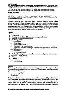
C. Pneumatic tires Aside from aerodynamic and gravitational forces, all other major forces and moments affecting the motion of a ground vehicle are applied through the running gear-ground contact. An understanding of the basic characteristics of the interaction between the running gear and the ground is, therefore, essential to the study of performance characteristics, ride quality, and handling behavior of ground vehicles. However, a detailed explanation about pneumatic tires is out of the scope of this paper. The following figure shows a summary of the main forces, moments and angles that play a major role on the modeling of the pneumatic tire. Each one is associated with a corresponding local axis located at the center of the contact patch of the wheel. Traction (Fx), lateral (Fy) and normal (Fz) forces along X, Y and Z local axis respectively and overturning (Mx), rolling resistance (My) and aligning (Mz) torques along the same axis respectively are modeled in terms of the slip and the camber angles and the pneumatic characteristics. For more details about the fundamentals and the modeling of pneumatic tires see [14, 1, 12].
Ks Kt
Bs
pitch
Kt
h1 Kt Fy
δ Fx
Figure 1: Full car model. As also the four suspension subsystems are modeled as spatial multibody systems, joint models are necessary to link them to the chassis. The joints are represented as flexible instead of rigid using a pseudo spring-damper system with elastic and damping constants. The flow and efforts actuating on the joints depend on the relative position and the relative orientation among the bodies. In order to link two rigid bodies at a given joint it is necessary to do some transformations (translations and rotations) between the reference frames associated to each body. In this way, the state variables expressed at the center of mass of each body are transformed to a local reference frame attached to the joint. B. Engine and Transmission Most vehicles are propulsed by internal (spark or compression ignited) combustion engines which -for our modeling purposes- may be modeled through a given static curve relating the engine speed and the load with its torque and its power. Usually, these curves are obtained through testing the engine at partial and full load. The transmission is composed by the mechanical members connecting the engine crankshaft with the traction wheels, the gearbox and the planetary gear train including the differential [8]. The main phenomena taken into account are the speed and effort transformation among them.
Figure 2: Tire axis reference system D. Suspensions Suspension is the term given to the system of springs, shock absorbers and linkages that connects a vehicle to its wheels. This assembly is used to support weight, absorb and dampen road shock, and help maintain tire contact as well as proper wheel-to-chassis relationship. Without being a restriction for future extensions of the overall vehicle model, only static suspension systems are considered in this work. E. Aerodynamic forces The aerodynamic forces were very simplified in this analysis through the usage of empirical aerodynamic coefficients [1, 16, 17]. In this work only the drag force was included, being the lift and the pitching effects very similar in terms of their mathematical expressions. In the future not only the coefficients, also their sensitivity may be included. III. MATHEMATICAL AND BG MODELING This section presents the subsystem modeling according to the hypothesis of Section II. Previously, the essential issues concerning the bond graph modeling of multibody systems as
used in this paper are addressed. To determine the spatial motion of the rigid body the well known Euler equations are used [2], which appear in (1) and (2) in both, their intrinsic way of representation and their tensorial counterparts. The first one represents the conservation of linear momentum, written as: dp dp ∑ F = dt = dt + ω × p (1) rel Fi =
dpi dpi = dt dt
dhi dhi = dt dt
M = F ×r
+ ε ijk ω j p k
(3)
M i = ε ijk F j rk
rel
where F , ω , p represents the external forces, the angular velocity vector and the linear momentum vector respectively; d/dt, d/dt|rel, εijk represent the derivative respect to the inertial frame, the derivative respect to the body (vehicle) attached frame and the Levi-Civita tensor used to express the cross product in tensor notation. The second of the Euler equations sets up the conservation of angular momentum: dh dh ∑ M = dt = dt + ω × h (2) rel Mi =
to the system attached to the center of mass of the rigid body. Referring these port variables to the coordinates of interconnection to other bodies is a must in order to be able to couple the corresponding models. Figure 4 shows the bond graph implementation of the equation system representing how the port variables of two arbitrary points 'A' and 'B' of a given spatial body transform each other. The equations relating the linear and rotational efforts are the following:
For the flow variables the equations are the following: v =ω ×r
(4)
vi = ε ijk ω j rk
+ ε ijk ω j hk rel
where M , h represent the external torque and the angular momentum vector.
Figure 4: Power variables transformation between two points ‘A’, ‘B’ belonging to a given 3-dimensional rigid body. To transform the dynamic equations from those expressed in the body attached frame of reference (roll, pitch and yaw axes) to a spatially fixed frame of reference (X,Y,Z : inertial frame) it is necessary to choose some parameterization for the rotations. Among the multiple possibilities, Euler angles are used in this work. To transform these rotations the following equations are used:
ω ′′ = φ × ω (5.a); ω ′ = θ × ω ′′ (5.b); ϖ G = ψ × ω ′ (5.c) v ′′ = φ × v (5.d); v ′ = θ × v ′′ (5.e); v G = ψ × v ′ (5.f) where,
Figure 3: BG representation of the spatial rigid body dynamics. The BG representation of the 3-dimensional motion of a rigid body based on the Euler equations is shown in figure 3. The port variables of the above model are defined with respect
0 ⎡1 ⎢ φ = ⎢0 cos φ ⎢⎣0 sin φ
⎤ − sin φ ⎥⎥ cos φ ⎥⎦ 0
⎡cosψ ψ = ⎢⎢ sinψ ⎢⎣ 0
⎡ cos θ θ = ⎢⎢ 0 ⎢⎣− sin θ − sinψ cosψ 0
0⎤ 0⎥⎥ 1⎥⎦
0 sin θ ⎤ 1 0 ⎥⎥ 0 cos θ ⎥⎦
⎡ω x ⎤ ω = ⎢⎢ω y ⎥⎥ ⎢⎣ω z ⎥⎦
⎡ω ′x′ ⎤ ω ′′ = ⎢⎢ω ′y′ ⎥⎥ ⎢⎣ω z′′ ⎥⎦
⎡ ω ′x ⎤ ⎡ω X ⎤ ω ′ = ⎢⎢ ω ′y ⎥⎥ ω G = ⎢⎢ωY ⎥⎥ ⎢⎣ω z′ ⎥⎦ ⎢⎣ω Z ⎥⎦
⎡v x ⎤ v = ⎢⎢v y ⎥⎥ ⎢⎣v z ⎥⎦
⎡v ′x′ ⎤ v ′′ = ⎢⎢v ′y′ ⎥⎥ ⎢⎣ v ′z′ ⎥⎦
⎡v ′x ⎤ v ′ = ⎢⎢v ′y ⎥⎥ ⎢⎣v ′z ⎥⎦
⎡v X ⎤ v = ⎢⎢ vY ⎥⎥ ⎢⎣ v Z ⎥⎦ G
Its bond graphs representation is observed in figure 5, where the power variables are transformed from (x,y,z) axes to the rotated ones (X,Y,Z) according to the angles φ, θ, ψ respect to each axis. It may be observed that while the flow variables are rotated from (xyz) to (XYZ), the effort variables are transformed back from (XYZ) to (xyz). Next, the models used for the different subsystems belonging to the whole vehicle model are presented [2, 12].
Figure 5: 3D-rotation equations expressed in terms of power variables.
Figure 6: BG modeling of Vehicle Chassis A. Vehicle Chassis Figure 6 shows the vehicle chassis model composed by a rigid body model, a coordinate system transformation to the global system where the vehicle weight is imposed and four translational transformations ( ri ) to the pivots of the
modeled as an effort source (the engine output torque) variable with the engine velocity normally expressed in rpm (revolutions per minute) and the position of the butterfly valve (accelerator command) as written by equation (6). T (T p , Tr , A p ) = A p T p (ω ) + (1 − A p ) Tr (ω )
(6)
suspension at each wheel, each one with their corresponding model Engine and Transmission
where Ap is the accelerator position (0 ≤ A p ≤ 1) , Tp and Tr
B. Engine and Transmission Engine. In bond graphs representation the engine is
are the engine output torque and the resistant torque respectively for a given engine speed (ω ) .
While the engine curve, the accelerator position and the resistant torque are data for the model, the engine speed is computed by the whole model. In the ‘Engine Torque’ model show in figure 7 the output torque is computed by equation (6) and its result T is used to modulate the source ‘MSe’.
input and output effort variables through a variable transformation factor that depends on the gearbox ratios supplied to the model in advance.
Figure 9: BG modeling of Gearbox
Figure 7: BG modeling of Engine
The differential (figure 10) is modeled by a transformer (TF) modulated by the planetary drive train (differential) ratio. The ‘0’ junction imposes the same torque to both traction wheels.
Figure 10:BG modeling of Differential
Figure 8: BG modeling of Transmission
C. Pneumatic Tires For all forces and moments acting on the tire the Pacejka model [14], inspired by a lot of experiments carried out using different types of pneumatic tires is used. µ x = sign(σ ) ⋅ ⎡ A ⋅ 1 − e− b σ + c ⋅ σ 2 − D ⋅ σ ⎤ ⎣ ⎦
(
)
B = (K / d )
1/ n
Transmission. Figure 8 shows the main components of the transmission and its structure. The gearbox (figure 9) is modeled using a modulated transformer (MTF) that relates the
A = 1.12 ; C= 0.625 ; D = 1 K = 46 ; d = 5 ; n = 0.6
(7)
This model is briefly described with the expressions (7), with -1< σ