Proc. 2nd Int. Workshop on Manufacturing and Petri Nets, Toulouse, June 1997, held at Int. Conf. on Application and Theory of Petri Nets (ICATPN ‘97), pp. 69 - 84.
VERIFICATION AND OPTIMIZATION OF CONTROL PROGRAMS 1) BY PETRI NETS WITHOUT STATE EXPLOSION Monika Heiner Brandenburg University of Technology at Cottbus Computer Science Institute Postbox 101344 D-03013 Cottbus
[email protected] http://www.informatik.tu-cottbus.de
Abstract: The development of provably error-free and efficient concurrent manufacturing systems is still a challenge of practical system engineering. Modelling and analysis of concurrent systems by means of Petri nets is one of the well-known approaches using formal methods. Among those Petri net analysis techniques suitable for strong verification purposes there is an increasing amount of promising methods avoiding the construction of the complete interleaving state space, and by this way the well-known state explosion problem. This paper demonstrates that available methods and tools are actually applicable successfully to at least medium-sized manufacturing systems. For that purpose, step-wise validation of various system properties (consistency, safety, progress) and optimization of the concurrent controller software of a discrete event system is performed. If possible, different analysis techniques are applied and compared with each other concerning their efforts. keywords: programmable logic controller, hierarchical place/transition nets, verification, optimization, temporal logics, model checking, interval nets;
1 Introduction Petri nets enjoy several advantages with respect to modelling and analysis of discrete event systems with inherent concurrency. Worth mentioning is especially the ability of combining different methods on a common representation. This variety ranges from informal (animation) via semi-formal (systematic testing) up to formal (exhaustive analysis) methods and comprises qualitative as well as quantitative evaluation techniques. But maybe most valuable is the fact that among the formal methods suitable for strong verification purposes there is an increasing amount of promising methods avoiding the construction of the complete interleaving state space, and by this way the well-known state explosion problem. This paper gives an overview on these alternative methods and reports our experience concerning their strength and limitations for verification and optimization purposes by a running example. The discussion covers 1) This work is supported by the German Research Council under grant ME 1557/1-1.
97/11/07
1 / 16
Verification and Optimization of Control Programs by Petri Nets without State Explosion
Title
• static analysis techniques, constructing no state space at all, • compression techniques, representing the transition relation by its characteristic function, • lazy state space construction, building reduced (interleaving) state spaces, which are generally much smaller than the complete state space for highly concurrent systems, • alternative state space construction, exploiting concurrency to build partial order (true concurrency) descriptions of the system behaviour. Beyond the more sophisticated (but scalable) running example, it is claimed that the optimistic analyses results are typical for a certain class of practical problems. This assumption is justified by case studies performed at our institute (see e.g. [10], short version in [11]), in which Petri net specifications of controller software of realistically sized production cells were developed. Step-wise validation processes were done in two stages: First, context checking (general analysis) of general semantic properties (mainly freedom of deadlocks, liveness and boundedness) was managed. Second, verification of well-defined special semantic properties, progress as well as safety properties, given by a separate requirement specification, was performed (special analysis). As widely accepted, temporal logics are a suitable tool to express such properties. For the evaluation of temporal logic formulae, the model checking approach is preferable to proof techniques in the case of finite state systems. In this paper, we deal mainly with qualitative analysis techniques suitable for place/transition nets without time constraints. Quantitative analyses are considered only to prove the unreachability of explicit error states. More detailed quantitative evaluations of our case studies, e. g. by different types of time-dependent Petri nets to prove the meeting of given deadlines in the framework of worst-case evaluation, and by stochastic nets to estimate throughput or average processing time, are in preparation. The running example is an adopted version of the pusher problem for which in [18] a control program has been synthesized automatically. By this way, this paper presents a reversal check for that synthesis. General transformation rules are sketched to transform programmable logic controller (plc) programs into ordinary place/transition Petri nets. Therefore, the rich amount of available Petri net analysis techniques and tools can be applied for computer-aided analysis of programmable logic controller programs. The paper is organized as follows. Section 2 gives a quick review on Petri net related analysis techniques which were used in our case studies. In section 3 and section 4, the running example and its informal requirement specification is introduced. Afterwards, the chosen way of modelling with hierarchical Petri nets is demonstrated in section 5. The validation of qualitative properties is described in more detail in section 6, while the necessity of handling quantitative properties in case of explicit error states is highlighted in section 7. Both analysis steps may take advantage of an optimization step. Related results are summarized in section 8. Finally, some conclusions are summarized in section 9.
2 Techniques and Tools Concerning methods for the analysis of Petri nets, animation, static techniques, and dynamic techniques can be distinguished.
2 / 16
[email protected]
Proc. 2nd Int. Workshop on Manufacturing and Petri Nets, Toulouse, June 1997, held at Int. Conf. on Application and Theory of Petri Nets (ICATPN ‘97), pp. 69 - 84.
Net-based animation aims at functional behaviour simulation by playing the token game. The results gained depend on the abstraction level of the underlying net model. But in any case, this special version of prototyping is only a confidence-building approach unable to replace exhaustive analysis methods. All static analysis techniques have in common that they avoid the enumeration of the state space of a system. The integrated net analyser INA [21] provides an almost complete collection of static analysis techniques of the “classical” Petri net theory [20]. Basic techniques corresponding mainly to general analysis (of boundedness or liveness) are reduction (local reduction rules to minimize the net structure) and structural analysis (structural properties allowing conclusions on behavioural properties, e.g. deadlock trap property). In opposite to that, linear-algebraic analysis revealing invariants supports general analysis (if the net is covered with semipositive place/transition invariants) as well as special analysis. In the latter case, program invariants are proven by showing the existence of related net invariants. So first, suitable program invariants have to be hypothesized, and second, the related net invariants have to be found from the (in general non-minimal) basis of invariants provided by a net analysis tool. Generally, this is hardly manageable for larger systems (larger concerning the size of states). Recently, new approaches appeared to combine invariant analysis techniques with an analysis of traps and model checking algorithms as well [13], [15]. If a desired system property can not be determined by structural analysis techniques, dynamic analyses may be applied. The classical approach is the exhaustive construction and exploration of the (interleaving) state space (reachability graph). INA provides the determination of general net properties like the freedom of deadlocks, boundedness, and liveness based on reachability analysis. More sophisticated analysis tasks can be formulated in the query language of the reachability graph analysis tool PROD [25]. Computational Tree Logic (CTL)1) is completely expressible in this language. Although almost every behavioural property of a Petri net with finite reachability graph can be theoretically decided by exhaustive analysis, this approach is limited in practice due to the state explosion problem. Compression techniques alleviate the state explosion by avoiding an explicit representation of the (interleaving) state space of a concurrent system. Ordered binary (or natural) decision diagrams (OBDDs, ONDDs) [2], [13] represent sets of states (and sets of transitions between states) by their characteristic function. Model checking (in this context sometimes called symbolic model checking) of temporal logic formulae can be performed on OBDDs (ONDDs) without an explicit enumeration of the state space state by state. Symbolic model checking was not considered yet in the validation of our case study examples, but is in preparation based on the ideas outlined in [26]. For an experience report of this approach see in the meantime e.g. [3]. For some analysis questions, it is only necessary to construct a reduced version of the interleaving state space of a system instead of the complete one. If we deal with system properties which are invariant under the interchanging of concurrent transition occurrences, it is unnec1) For an introduction to temporal logics and the notation used in this paper see [5].
97/11/07
3 / 16
Verification and Optimization of Control Programs by Petri Nets without State Explosion
Title
essary to consider all those interleavings. In this way, dead states for instance can be found or the un-/reachability of special states can be decided by considering an usually small subset of all possible interleaving paths. Methods based on this idea are sometimes called partial order methods (a term which should be sharply distinguished from partial order representation techniques described below). An example of a partial order method is Valmari’s stubborn set method [23]. The stubborn set method can be combined with other techniques like the sleep set method [9], and the symmetry method [24]. Valmari developed a generalization of his method in a way that properties expressible by Linear Temporal Logic (LTL) without the nexttime operator X are preserved by the reduction process. Therefore, the standard model checking technique for LTL can be applied to stubborn reduced reachability graphs. Besides its model checking facilities for CTL, PROD provides a LTL model checker based on this approach. The basic stubborn set method for deadlock detection is also implemented in INA. An alternative class of approaches to handle the state explosion problem bases on partial order representations of the behaviour of a concurrent system. Instead of sequences of events (i. e. occurrences of transitions), partially ordered sets of events are used as behaviour description. Partial orders of events can be interpreted in the following way: If an event precedes another one then the former one causes the latter, or the former one has to occur earlier in time than the latter. Since state explosion is in general caused by the representation of all possible interleavings of concurrent actions, partial order representations tend to be much smaller than reachability graphs. A currently intensively discussed partial order representation approach is the construction of a “finite complete prefix of a branching process” of a Petri net (shortly called the prefix of the net) [6], [14]. The possible behaviour of the net is represented by another, so-called occurrence net. The PEP tool [1], [7] provides, besides many other things, an efficient model checking algorithm based on this net prefix for a very restricted subset of CTL comprising only the temporal operators AG and EF. This model checker is restricted to safe (1-bounded) Petri nets. Which tools should be applied in which order depends on the analysis methods they are based on. Which tools may be applied at all for a given type of question depends on their power to express a specific analysis question. To highlight differences between the applied tools concerning their expressiveness, it is useful to summarize typical questions/properties dealt with during analysis. In the following ϕ stands shortly for a general logical expression characterizing usually a (wanted or unwanted) state or set of states. (1)
reachability-related properties of the logical form EF ϕ : Reachability of a state where ϕ holds; there exists at least one computation path (future behaviour) to reach eventually a state where ϕ will be true.
(2)
safety-related, AG ( ¬ϕ ) or equivalent ¬EF ϕ : Unreachability of a state where ϕ holds; for every computation path, ϕ will never be true.
(3)
invariant-related, AG ϕ or equivalent ¬EF ( ¬ϕ ) : General validity of an assertion ϕ; for every computation path, ϕ will be true for ever.
(4)
liveness-related, AG EF ϕ : What ever happens, there exists the chance (at least one path) that ϕ will be true.
4 / 16
[email protected]
Proc. 2nd Int. Workshop on Manufacturing and Petri Nets, Toulouse, June 1997, held at Int. Conf. on Application and Theory of Petri Nets (ICATPN ‘97), pp. 69 - 84.
(5)
progress-related, AG AF ϕ : For every computation path, ϕ will eventually be true.
Table 1 describes which tool may be applied for which type of logical expression. Table 1: Temporal operators provided by the different tools.
Supported type of logic
Tool
Types of properties
Operators
INA
-
EF ϕ (but ϕ can only be given by a (sub-) marking)
(1), (2)
PEP
(restricted) CTL
AG, EF
(1) - (4)
PROD
LTL (without nexttime operator)
G, F, U (unquantorized versions of AG, AF, AU)
(2), (3), (5)
PROD
(full) CTL
EX/AX, EF/AF, EG/AG, EU/AU
(1) - (5)
The tool kit used up to now comprises PED (hierarchical Petri net editor) [16], INA (structural properties, place/transition invariants, stubborn set reduced deadlock and reachability analysis, net reductions) [21], PROD (stubborn set reduced deadlock analysis and model checking LTL\X) [25], and PEP (prefix-based model checking - CTL0, linear-algebraic analysis) [1]. More details can be found in the related tool manuals.
3 Task Description
Controller 2 M
Pos. 2
R1
Pos. 3
R2
Pusher 2 Piece, Pos. 1 Pusher 1
The example consists basically of two concurrently working pushers moving work pieces (see figure 1). The work piece is moved from position one to position two by the first pusher, and from position two to position three by the second pusher. Both pushers are driven by electric motors which can be controlled by corresponding relays into two moving directions.
R2
Figure 1: Plant.
M Controller 1 R1
To make the paper self-contained, the running example, adopted from [18], is shortly sketched.
Starting from this basic situation, chains of concurrent pushers may be constructed in order to move pieces step by step from the input position via a number of inner positions to the output position.
97/11/07
5 / 16
Verification and Optimization of Control Programs by Petri Nets without State Explosion
Title
4 Requirement Specification In addition to the task description given above, a list of informally specified safety and progress properties is provided. Typical properties of this type are: (a) safety • At any time, a pusher can be driven in one direction only. • To avoid collisions, it is not allowed to move adjacent pushers at the same time. • No pusher motion must be driven too far/near. • While moving a pusher, a new work piece must not arrive in its input position. (b) progress • After an active phase of a pusher, its successor will be activated before the predecessor will be started again. • It is guaranteed that each pusher works infinitely often (livelock freedom). • Any work piece entering the plant will finally leave the plant. (c) consistency • Additional properties to be verified emerge during modelling reflecting useful (self-) consistency checks (see section 5.1).
5 Modelling with Hierarchical Petri Nets The model of the total system may be characterized by a strong separation of controller software and environment into different parts. The controller program consists generally of a finite and static set of communicating processes. The environment model is composed of small reusable components: the producer/consumer processes of the work flow, and the devices of the controlled plant.
controller
producer
consumer
actuators
sensors
plant environment
The composite model is structured into three layers. The top layer of a transport system with two pushers (Figure 2) consists of six macro components. Each macro transition P1 and P2 contains the plant environment model given in Figure 3, but prefixed with the instance names P1 or P2, respectively (see section 5.1). Each macro transition con1 and con2 contains the controller software model sketched in Figure 4, but prefixed with the instance names C1 or C2, respectively (see section 5.2).
5.1 Environment Model There exists a net component for each device type - building step-by-step a growing reusable
6 / 16
[email protected]
Proc. 2nd Int. Workshop on Manufacturing and Petri Nets, Toulouse, June 1997, held at Int. Conf. on Application and Theory of Petri Nets (ICATPN ‘97), pp. 69 - 84.
Figure 2: Top layer of a transportation system with two pushers. pos1_full
pos2_full
pos3_full
Drawing convention: producer
con1
pos1_free
pos2_free
P1
consumer
con2
Shadowed nodes are so-called logical (fusion) nodes. They serve as connectors to avoid immoderate edge crossing. All logical nodes with the same name are logically identical.
pos3_free
P2
component library to describe the uncontrolled plant behaviour. Each physical device is basically characterized by its finite set of discrete states (maybe representing equivalence classes of possibly infinite sets of states), and additionally by the commands (externally visible transitions - the grey ones) forcing the device to change its current state (see fig. 3). Obviously, each device must be in one and only one state at any time. In terms of Petri net theory, the states of a device form a place invariant. In our example, there are two types of devices (relays, pushers). Accordingly, there are two consistency conditions. E.g. it holds for all pushers Pi: (P1) ( Pi_too_near + P i_basic + Pi_norm + Pi_ext + Pi_too_far ) = 1 . or expressed as temporal formula ( ∨ stands for exclusive or): . . . . (P1*) AG ( Pi_too_near ∨ Pi_basic ∨ Pi_norm ∨ Pi_ext ∨ Pi_too_far ) For a more systematic analysis procedure (see section 6 and section 7), two versions of pushers are considered: without and with explicit error states (too_near, too_far). In the initial state (marking), all relays are off, the pushers are in their basic positions, and the plant is empty (contains no work piece).
Figure 3: Components of the uncontrolled plant environment model. RELAY R1
PUSHER
R1_set_on
R1_on
with error states
R1_on R1_set_off
basic2norm
norm2ext
ext2far
too_nearF R1_off
RELAY R2
too_near
norm
basic
ext
too_far
R2_on R2_set_on
R2_set_off
basic2near
norm2basic
ext2norm
too_farF
R2_off R2_on
97/11/07
7 / 16
Verification and Optimization of Control Programs by Petri Nets without State Explosion
Title
5.2 Control Program Model The pattern of the essential parts of the controller macro transitions (con1, con2) is given in Figure 4. The original programmable logic controller programs are written in IEC 1131-3 [4] (see left part). These programs are (automatically1)) translated into ordinary place/transition nets. For an example, how this could look like, consider the right side in Figure 4. In order to avoid unnecessary restrictions of the concurrency degree, it could be helpful to exploit a special test arc feature for modelling of the transitions’ side conditions (in our running example: Ri_on, Ri_off. In that case, the amount of data, which has to be searched through during the analysis steps, may become much smaller, provided the analysis tools are prepared to handle test arcs (compare discussion in section 6.1).
Figure 4: Part of the unoptimized controllers’ program and its Petri net model. start_moving
start_moving
R1_off
LD R1_off AND basic AND posIN_full
tr1
basic
tr1
posIN_full BOOL R1_set_on N
Step 1 LD R1_on AND ext AND posOUT_full
step1
R1_set_on R1_on
tr2
ext
tr2
posOUT_full Step 2 LD R1_off AND ext AND R2_off
BOOL N
R1_set_off
step2
R1_set_off R1_off
tr3
ext
tr3
R2_off BOOL N
Step 3
R2_set_on
step3
R2_set_on R2_on
LD R2_on AND basic
tr4
tr4 BOOL N
Step 4 R2_off
R2_set_off
basic
step4
tr5
R2_set_off R2_off
tr5
stop_moving
stop_moving
Macro: R1_set_on
Macro: R1_set_off
step1
step1
R1_off
R1_remains_on
R1_set_on R1_on
R1_on
R1_on
R1_remains_off
R1_set_off
R1_off
R1_off step1
step1
1) The automatization of this translation is part of the running project.
8 / 16
[email protected]
Proc. 2nd Int. Workshop on Manufacturing and Petri Nets, Toulouse, June 1997, held at Int. Conf. on Application and Theory of Petri Nets (ICATPN ‘97), pp. 69 - 84.
5.3 Requirement Specification in Model Terms Finally, the informally given requirement specifications have to be transformed into the terms of the formal model. (a) safety • At any time, a pusher can be driven in one direction only: (P2)
AG ( ¬( Pi_R1_on ∧ Pi_R2_on ) ) , ∀i
• To avoid collisions, it is not allowed to move adjacent pushers at the same time:
(P3)
2 2 Pj_Ri_on + Pk_Ri_on ≤ 1 , ∀i, ∀ j, k : j + 1 = k i = 1 i=1
∑
∑
• No pusher motion must be driven too far/near: (P4)
AG ( ¬Pi_too_near ) , ∀i
(P5)
AG ( ¬Pi_too_far ) , ∀i
• While moving a pusher, a new work piece must not arrive in its input position: (P6)
AG ( posi_full → Pi_basic ) , ∀i
(b) progress • After an active phase of a pusher, its successor will be activated before the predecessor will be started again: (P7)
AG ( Pi_norm ∨ Pi_ext → ) AF ( ¬( Pi_norm ∨ Pi_ext )AU ( Pj_norm ∨ Pj_ext ) ) ) , ∀i, j : i + 1 = j
• It is guaranteed that each pusher works infinitely often (livelock freedom), e.g. (en(t) stands for the conjunction of all preplaces of t): (P8)
AG ( AF ( en ( Pi_basic2norm ) ) ) , ∀i
• Any work piece entering the plant will finally leave the plant (which may be considered as a consequence of (P7) and (P8)), i.e. in case of a two-pushers chain: (P9)
AG ( pos1_full → AF pos3_full )
6 Qualitative Analysis We present a two-step analysis. At first, the pusher model without explicit error states is discussed in this section. Afterwards, the error states are integrated leading to the notion of time (see section 7).
97/11/07
9 / 16
Verification and Optimization of Control Programs by Petri Nets without State Explosion
Title
6.1 General Analysis General analysis deals with properties which should be valid independently of the intended functional behaviour of the system. Basically, these are boundedness and liveness. boundedness: The net is covered by semi-positive place invariants (INA). Moreover, the token sum of all these place invariants equals to 1. So we are able to conclude the 1-boundedness of the net (a necessary precondition for PEP’s model checker). liveness: The deadlock freedom can be proven very efficiently by construction of stubborn reduced reachability graphs (INA, PROD), which are generally much smaller than the complete state space. Additionally, it can be shown efficiently that the net is covered by semi-positive transition invariants as necessary (but not sufficient) condition for liveness. But liveness (no dead system parts) can’t be proven by classical Petri net theory for longer pusher chains, due to the lack of suitable net structures (the given nets are not Extended Simple, therefore the deadlock trap property could not help, the known local net reduction rules do not work), and due to the state explosion by considering all interleaving transition sequences (reachability graph). The way-out could be a liveness proof for each transition by model checking the temporal formula: AG EF ( en ( t ) ) based on the branching process’ prefix. However (compare Table 2), the prefixes are also unconstructable for more than 6 pushers. The reason for that seems to be the dynamic conflicts caused by the right-hand transitions in the macros of Figure 4, bottom - Ri_remains_on, Ri_remains_off). After having switched on/off the corresponding relay, they are reproducing the current state until the control program goes ahead (because the pusher has reached the position the controller is waiting for). Due to the lack of test arcs to model side conditions, these reproductions are done in an active way resulting into “useless” dynamic conflicts. These dangerous transitions are part of general net components for context-independent modelling of basic statements (here to switch the relay on/off). Obviously, such a statement is actually executed in finite time independently of the current situation, i.e. whether the relay is already on/off. The same should hold for an appropriate model of that basic statement. Therefore we need generally these transitions under discussion within the corresponding macro transitions to model adequately both situations. But in case of the given Petri net, modelling a programmable logic control program, these basic statements appear (only) as side conditions of the control flow, and never within the control flow. That’s why these transitions are superfluous in the given case, and we are able to optimize our model by deleting them. We get a first version of an optimized model with the same state space as the unoptimized one (compare the third columns of Table 2 and Table 3), but without far less dynamic conflicts. For this version, the liveness for each transition of the considered pusher chains has been proven by model checking the corresponding temporal formula based on the branching process’ prefix.
6.2 Special Analysis (a) safety
10 / 16
[email protected]
Proc. 2nd Int. Workshop on Manufacturing and Petri Nets, Toulouse, June 1997, held at Int. Conf. on Application and Theory of Petri Nets (ICATPN ‘97), pp. 69 - 84.
There are different analysis techniques available to prove the unreachability of unsafe states (P2) - (P6): Facts (INA): The unsafe states may be modelled as facts (special transitions which are expected to become never enabled). But, the evaluation of bad states (a state where a fact is enabled) by the given tool kit requires the reachability graph. That’s why we will avoid this approach. Stubborn set reduction (INA): The net is transformed in such a way that the unsafe states become dead states. Then the stubborn set reduced reachability graph has to be constructed. Because any dead states are preserved under this reduction, the original net does not contain any unsafe states if the transformed net does not reach any dead states. This technique could be useful if the required net transformation is done by the analysis tool. Place invariants (INA): A sufficient condition for the unreachability of a given marking m is fulfilled if the there exists at least one place invariant x for which the token conservation equation ∑ x ( p ) ⋅ m0 ( p ) = ∑ x ( p ) ⋅ m ( p ) p∈P p∈P is not valid. To check this equation, complete markings must be specified. But unsafe states are usually given in terms of submarkings (containing “don’t care” places). This main disadvantage is overcome in the next approach. Trap equation (PEP): Based on a linear upper approximation of the state space, a sufficient condition for linear properties of the type A ⋅ m ≤ b has been introduced in [15]. The implementation is integrated in the latest version of PEP. We use it to prove (P3). Model checking of temporal formulae: Model checking, combined with stubborn set reduction (PROD, LTL\X) or based on the finite complete prefix of a branching process (PEP, CTL0), provides generally the most convenient method to raise safety questions, esp. because set of (unsafe) states may be characterized in a concise manner. Both model checkers run very fast. Due to the evaluation method, they are applicable also to larger systems of which the size of the interleaving state space is unknown. (b) progress (P7) - (P9) use a richer set of (temporal) logical operators. Therefore, model checking facilities are unavoidable. Due to the AF and AU operators, these properties can be proven only by PROD. We use it to prove (P7) - (P9) for any pusher chain. (c) consistency For any pusher chain, (P1) is analyzable by INA, and in the version of (P1*) by PROD or PEP. But for larger systems, it is generally a cumbersome task to prove this type of properties by finding the suitable place invariants. A summary on the analysis efforts necessary to gain the results mentioned above are given in
97/11/07
11 / 16
Verification and Optimization of Control Programs by Petri Nets without State Explosion
Title
the tables 2 and 3. Table 2: Overview on analysis efforts of the unoptimized model. # pushers
P/T
R
Rstub
prefix (B / E)
time(prefix)a)
1 2 3 4 5 6 7 8 9 10
24 / 25 42 / 46 60 / 67 78 / 88 96 / 109 114 / 130 132 / 151 150 / 172 168 / 193 186 / 214
88 464 3.088 18.848 118.624 738.368 4.614.208 ? ? ?
22 42 79 133 204 292 397 519 658 814
128 / 61 293 / 139 510 / 242 779 / 370 1100 / 523 1473 / 701
0:0.02 0:0.08 0:0.40 0:3.08 0:43.14 11:38.86
b)
a) SUN SPARC 20, 32 Mbyte main memory b) memory overflow after about 50 min having allocated 120 Mbyte main memory.
Table 3: Overview on analysis efforts of the optimized model. # pushers
P/T
R
Rstub
prefix (B / E)
time(prefix)
1 2 3 4 5 6 7 8 9 10
24 / 21 42 / 38 60 / 55 78 / 72 96 / 89 114 / 106 132 / 123 150 / 140 168 / 157 186 / 174
88 464 3.088 18.848 118.624 738.368 4.614.208 ? ? ?
22 42 79 133 204 292 397 519 658 814
96 / 45 213 / 99 366 / 170 555 / 258 780 / 363 1041 / 485 1338 / 624 1671 / 780 2040 / 953 2445 / 1143
0:0.02 0:0.05 0:0.15 0:0.36 0:0.63 0:1.19 0:1.97 0:3.54 0:5.26 0:6.93
7 Quantitative Analysis In case of explicit error states within the model (Pi_too_far, Pi_too_near), it has to be proven that a pusher, after having reached the expected extension, is switched off fast enough. Obviously, we have now to take into consideration also the timing behaviour of the given system. In terms of interval Petri nets [12], [17] (usually called time Petri nets) this means that the error transitions modelling the pusher motions into unsafe states (Pi_ext2far, Pi_basic2near) may be enabled, but will never fire due to the influence of time. Therefore, the proof of the unreachability of explicit error states ((P4), (P5)) can be traced back to the proof that the related error transitions are dead at the initial state.
12 / 16
[email protected]
Proc. 2nd Int. Workshop on Manufacturing and Petri Nets, Toulouse, June 1997, held at Int. Conf. on Application and Theory of Petri Nets (ICATPN ‘97), pp. 69 - 84.
This may e.g. happen because the transitions Ci_tr2 and Pi_R1_set_off (disabling Pi_ext2far) fire always before Pi_ext2far is willingly to fire (compare figure 5) showing the essential part of the condensed reachability graph). Generally, a proof like that depends essentially on the chosen interval times (but can be done by INA, at least as long as the reachability graph fits into memory). But in this concrete case, we are able to conclude - by evaluating a suitable part of the reachability graph (or at best a non-interleaving version of it) - that for any time intervals for which the relations lft ( Ci_tr2 ) < eft ( Pi_ext2 far ) ∧ lft ( Ri_set_off ) < eft ( Pi_ext2 far ) hold, the dangerous transitions Pi_ext2far will never fire. Similar relations hold for Pi_basic2near.
Figure 5: Part of the condensed reachability graph.
C_init, R1_off, P1_basic tr1; R1_set_on; step1, R1_on, P1_ext
P1_ext2far
step1, R1_on, P1_too_far
bad state!
step2, R1_on, P1_too_far
bad state!
tr2 step2, R1_on, P1_ext
P1_ext2far
R1_set_off; tr3
step3, R1_off, P1_ext
Remark: Only the interesting parts of the markings are shown.
8 Optimization By help of provably correct optimization assumptions, the amount of side conditions at the transitions in the synthesized controller program may be minimized, e.g.: • Because ext always implies PosOUT_full: (P10)
AG ( ext → Po sOUT_full )
at transition tr2 the side condition PosOUT_full could be deleted. • Because step2 always implies R2_off: (P11)
97/11/07
AG ( step2 → R2_off )
13 / 16
Verification and Optimization of Control Programs by Petri Nets without State Explosion
Title
at transition tr3 the side condition R2_off could be deleted. Of course, code optimization must not destroy any requirement property just proven. Therefore, regression verification has to be done in the background as the final validation step.
9 Conclusions At least for the analysis of a restricted class of concurrent systems modelled by Petri nets, the construction of the complete state space can be avoided by a suitable combination of different methods (possibly implemented by different tools). This class can be characterized as follows: • (Intentionally) life and 1-bounded systems (hence, covered by semipositive place and transition invariants), • a certain degree of concurrency (which increases the efficiency of partial order methods and partial order representation methods), • moderate amount of dynamic conflicts. So, all qualitative (i.e. timeless) properties and optimization assumptions have been proven without construction of the reachability graph (interleaving state space). Up to now, the quantitative (i.e. time-dependent) analysis of interval nets is based on reachability graph construction and evaluation. But in [19], a method has been proposed to describe the behaviour of interval nets by a finite prefix of branching processes. It seems to be worth thinking over how to combine both approaches. Nevertheless, all proves were carried out automatically by help of general Petri net analysis tools. Therefore, they are reproducible in an objective way. For a general framework for Petri net based development and analysis, we conclude the following design criteria. At first, dedicated technical languages are needed to express functional, safety, and performance requirements as well. Second, the framework has to be customizable. Its components (editors, analysis tools, simulation tools, code generation facility) should be interchangeable. For a given configuration, user guidelines are required showing which analysis techniques are recommendable in which order for a given analysis question. Additionally, design criteria are required which promotes meaningful analyses at each phase of development. For specific application areas, dedicated configurations of the framework can be defined involving also an adaptation of the libraries and the terminology of the user interface. For instance, in manufacturing control in general, it seems to be possible to compile Petri net libraries of • patterns which describe the communication structure of certain devices on a cooperation level (for the production cell of our case study [11], three such patterns are identifiable, each of them applicable to at least two devices), • patterns which are suitable to describe elementary motion steps of the devices, and • the associated environment models. Using these libraries, control programs for the supported types of manufacturing systems can be developed by composition and refinement of instantiated net patterns.
14 / 16
[email protected]
Proc. 2nd Int. Workshop on Manufacturing and Petri Nets, Toulouse, June 1997, held at Int. Conf. on Application and Theory of Petri Nets (ICATPN ‘97), pp. 69 - 84.
In particular, in case of programmable logic controllers, the user interface may be adapted to the notions of the IEC 1131-3 standard [4].
References [1] BEST, E.; GRAHLMANN, B.: PEP - Programming Environment Based on Petri Nets, Documentation and User Guide; Univ. Hildesheim, Dep. of CS, Nov. 1995, http://www.informatik.uni-hildesheim.de/pep/HomePage.html. [2] BRYANT, E. R.: Symbolic Boolean Manipulation with Ordered Binary-Decision Diagrams; ACM Computing Survey, 24(1992)3, 293-318. [3] CORBETT, J. C.: Evaluating Deadlock Detection Methods for Concurrent Software; Techn. Report, Dep. of Information and CS, Univ. of Hawaii at Manoa, 1995. [4] DIN IEC-1131-3: Pogrammable Logic Controller, Part 3: Programming Languages, 1994. [5] EMERSON, E. A.: Temporal and Modal Logic; in: J. v. Leeuwen, ed.: Handbook of Theoretical Computer Science, Vol. B; Elsivier, Amsterdam 1990, 995-1072. [6] ENGELFRIET, J.: Branching Processes of Petri Nets; Acta. Inf. 25(1991), 575-591. [7] ESPARZA, J.: Model Checking Using Net Unfoldings; Science of Computer Programming, 23(1994), 151-195. [8] GERTH, R., PELED, D., VARDI, M. Y., WOLPER, P.: Simple On-the-fly Automatic Verification of Linear Temporal Logic; Proc. of the 15th International Symposium on Protocol Specification, Testing and Verification (PSTV'95), Warsaw 1995, 3-18. [9] GODEFROID, P.: Partial-Order Methods for the Verification of concurrent Systems; LNCS 1032, 1996. [10] HEINER, M., DEUSSEN, P.: Petri Net Based Qualitative Analysis - A Case Study; BTU Cottbus, Dep. of CS, Techn. Report I-08/1995, http://www.informatik.tu-cottbus.de. [11] HEINER, M.; DEUSSEN, P.; SPRANGER, J.: A Case Study in Developing Control Software of Manufacturing Systems with Hierarchical Petri Nets; Proc. 1st Int. Workshop on Manufacturing and Petri Nets held at ICATPN ’96, Osaka, June ’96, pp. 177-196. [12] HEINER, M.; POPOVA-ZEUGMANN, P.: Worst-case Analysis of Concurrent Systems with Duration Interval Petri Nets; BTU Cottbus, Dep. of CS, Techn. Report I-02/1996, http://www.informatik.tu-cottbus.de. [13] LAUTENBACH, K.; RIDDER, H. A.: Completion of the S-invariance Technique by Means of Fixed Point Algorithms; Fachbericht Informatik 10/95, Univ. Koblenz-Landau, 1995. [14] MACMILLAN, K. L.: Using Unfoldings to Avoid the State Explosion Problem in the Verification of Asynchronous Circuits; Proc. of the 4th Workshop on Computer Aided Verification, Montreal 1992, 164-174.
97/11/07
15 / 16
Verification and Optimization of Control Programs by Petri Nets without State Explosion
Title
[15] MELZER, S.; ESPARZA, J.: Checking System Properties via Integer Programming; ESOP ’96, Linköping, LNCS 1058, pp. 250-264. [16] TIEDEMANN, R.: PED - Hierarchical Petri Net Editor, Manual (in German); BTU Cottbus, Dep. of CS, Internal Techn. Report, May 1997, http://www-dssz.Informatik.TU-Cottbus.De/~wwwdssz/ped.html. [17] POPOVA-ZEUGMANN, L.: On Time Petri Nets; J. Information Processing and Cybernetics EIK 27(91)4, pp. 227-244. [18] RAUSCH, M.; LÜDER; A.; HANISCH, H.-M.: Combined Synthesis of Locking and Sequential Controllers; Proc. WODES ’96, Edinburgh/UK, Aug. 1996, pp. 133-138. [19] SEMENOV, A.; YAKOVLEV, A.: Verification of Asynchronous Circuits Using Petri Net Unfolding; Proc. DAC ‘96, Las Vegas, June 1996, pp. 59-63. [20] STARKE, P. H.: Analysis of Petri Net Models (in German); Teubner, Stuttgart 1990. [21] STARKE, P. H.; ROCH, S.: INA - Integrated Net Analyzer Version 1.7, Manual (in German); Humboldt Univ. at Berlin, April 1997, http://www.informatik.hu-berlin.de/lehrstuehle/automaten/ina/. [22] VALMARI, A.: A Stubborn Attack on State Explosion; Formal Methods in System Design 1(1992)4, 297-322. [23] VALMARI, A.: Alleviating State Explosion during Verification of Behavioral Equivalence; Univ. of Helsinki, Department of Computer Science, Report A-1992-4, Helsinki 1992. [24] VARPAANIEMI, K.: On Computing Symmetries and Stubborn Sets; Helsinki Univ. of Technology, Digital Systems Laboratory, Series B, Report No. 12, Espoo 1994. [25] VARPAANIEMI, K. et al.: PROD Reference Manual; Helsinki Univ. of Technology, Digital Systems Laboratory, Series B: Techn. Report No. 13, August 1995, ftp://saturn.hut.fi/pub/reports. [26] WIMMEL, G.: A BDD-based Model Checker for the PEP Tool; Univ. of Newcastle, Dep. of CS, Major Individual Project, May 1997.
16 / 16
[email protected]