Verifying Fence Elimination Optimisations. Viktor Vafeiadis1 and Francesco Zappa Nardelli2. 1 MPI-SWS. 2 INRIA. Abstract. We consider simple compiler ...
Verifying Fence Elimination Optimisations Viktor Vafeiadis1 and Francesco Zappa Nardelli2 1
MPI-SWS INRIA
2
Abstract. We consider simple compiler optimisations for removing redundant memory fences in programs running on top of the x86-TSO relaxed memory model. While the optimisations are performed using standard thread-local control flow analyses, their correctness is subtle and relies on a non-standard global simulation argument. The implementation and the proof of correctness are programmed in Coq as part of CompCertTSO, a fully-fledged certified compiler from a concurrent extension of a C-like language to x86 assembler. In this article, we describe the soundness proof of the optimisations and evaluate their effectiveness.
1
Introduction
Contrary to a na¨ıve programmer’s expectations, modern multicore architectures do not implement a sequentially consistent (SC) shared memory, but rather exhibit a relaxed consistency model. For instance, x86 provides a TSO-like memory model [18, 23] while Power exhibits much more relaxed behaviour [19]. Programming directly against such relaxed hardware can be difficult, especially if performance and portability are a concern. For this reason, programming languages need their own higher-level memory model, and it is the role of the compiler to guarantee that the language memory model is correctly implemented on the target hardware architecture. Naturally, SC comes as an attractive choice because it is intuitive to programmers, and SC behaviour for volatiles and SC atomics is an important part of the Java and C++0x memory models, respectively. However, implementing SC over relaxed hardware memory models requires the insertion of potentially expensive memory fence instructions, and if done na¨ıvely results in a significant performance degradation. For instance, if SC is recovered on x86 by systematically inserting an MFENCE instruction either after every memory store instruction, or before every memory load (as in a prototype implementation of C++0x atomics [26]), then on some benchmarks (e.g. Fraser’s library of lock-free algorithms [11]) we could observe a 40% slowdown with respect to a hand-optimised implementation. Compiler optimisations to optimise barrier placement are thus essential, and indeed there are many opportunities to perform fence removal optimisations. For example, on x86, if there are no writes between two memory fence instructions, the second fence is unnecessary. Dually, if there are no reads between the two fence instructions, then the first fence instruction is redundant. Finally, by a form of partial redundancy elimination [17], we can insert memory barriers at
selected program points in order to make earlier fence instructions redundant, with an overall effect of reducing the number of fences along all execution paths and hoisting barriers out of a loop. However, concurrency, especially relaxed-memory concurrency, is a notoriously subtle and error-prone domain [10, 20], and so verifying such optimisations is of great interest. Work in this area goes back at least to that of Shasha and Snir [24] (and more recently [2, 6, 21]), but most of this is in terms of transformations of hypothetical program executions rather than the transformations of code that are implemented (without proof) in actual compilers. In this paper, we bridge this gap by implementing the aforementioned redundant barrier removal optimisations in CompCertTSO [22], a fully fledged verified compiler from ClightTSO (a C-like concurrent language with TSO semantics) to concurrent x86 assembly code with x86-TSO semantics. We prove the correctness of our optimisations in Coq and integrate this result into the overall semantic preservation proof of CompCertTSO, giving an end-to-end correctness result.3 The correctness result verifies that these fence removal optimisations do not introduce any new TSO behaviour. They are therefore sound in several different usages: for ClightTSO code with manually inserted fences; in a TSO implementation of a DRF-based memory model, such as C++0x [3] or the Java memory model [16], where fences are used to implement the language’s low-level atomic primitives; or if one implements SC by starting with a placement of fences admitting only SC-behaviours (e.g. by placing a fence after every memory write) and then optimises away as many as possible. The correctness of one of our optimisations turned out to be more much interesting than we had anticipated and could not be verified using a standard forward simulation because it introduces unobservable non-determinism (see §3 for an explanation). To verify this optimisation, we introduce weaktau simulations (see §4), which in our experience were much easier to use than backward simulations [15]. In contrast, the other two optimisations were straightforward to verify, each taking us less than a day’s worth of work to prove correct in Coq. Hence, we believe that developing mechanised formal proofs about concurrent optimising compilers offers a good benefit to effort ratio, once the right foundations are laid out. Outline. We begin, in §2, by recalling the relaxed-memory behaviour of our target architecture, as captured by the x86-TSO model, and the structure and correctness statement of the CompCertTSO verified compiler. Then, in §3, we describe our optimisations and their implementation in CompCertTSO, and evaluate their performace. In §4, we describe our overall simulation proof strategy for verifying compiler correctness, and in §5 the use of this strategy to verify the optimisations in question. Finally, in §6, we reflect on our experience using Coq and in §7 we discuss related work.
3
The proofs are available at http://www.cl.cam.ac.uk/~pes20/CompCertTSO/.
H/W thread
H/W thread
Write Buffer
Write Buffer
Lock
Shared Memory
Fig. 1. x86-TSO block diagram
2
The x86-TSO Memory Model & CompCertTSO
The x86-TSO model [18, 23] is a rigorous memory model that captures the memory behaviour of the x86 architecture visible to the programmer, for normal code. Figure 1 depicts the x86-TSO block diagram: each hardware thread has a FIFO buffer of pending memory writes (which can propagate to memory at any later time, thereby avoiding the need to block while a write completes); memory reads return the latest memory write pending in the thread write buffer, or, if there are no pending writes, the value written in the shared memory. Memory fences (MFENCE) flush the local write buffer: formally, they block until the buffer is empty. ‘Locked’ x86 instructions (e.g. LOCK INC) involve multiple memory accesses performed atomically. Such atomic read-modify-write instructions first block until the local write buffer is empty, and then atomically perform a read, a write of the updated value, and a flush of the local write buffer. The classic example showing a non-SC behaviour in TSO is the store buffer program below (SB). Given two distinct memory locations x and y initially holding 0, the memory writes of two hardware threads respectively writing 1 to x and y can be buffered, and the subsequent reads from y and x (into register EAX on thread 0 and EBX on thread 1) are fulfilled by the memory (which still holds 0 everywhere), and it is possible for both to read 0 in the same execution. It is easy to check that this result cannot arise from any SC interleaving, but it is observable on modern Intel or AMD x86 multiprocessors. If MFENCE instructions are inserted after the memory writes, as in SB+mfences, then at least one buffer must be flushed before any read is performed, and at least one thread will observe the write performed by the other thread, as in all SC executions. SB+mfences SB Thread 0 MOV [x]←1 MOV EAX←[y]
Thread 1 MOV [y]←1 MOV EBX←[x] Allowed final state: 0:EAX=0 ∧ 1:EBX=0
Thread 0 MOV [x]←1 MFENCE MOV EAX←[y]
Thread 1 MOV [y]←1 MFENCE MOV EBX←[x] Forbidden final state: 0:EAX=0 ∧ 1:EBX=0
CompCertTSO [22, 8] is a certified compiler that lifts the x86-TSO model of the x86 assembly language to a C-like language. Its source language, ClightTSO, is a concurrent extension of CompCert Clight language [4], adding thread creation and some atomic read-modify-write and barrier primitives that are directly implementable by x86 locked instructions and MFENCE. In addition, ClightTSO load and store operations have a TSO semantics. The main syntactic difference between Clight and C is that expressions cannot contain function calls and memory writes (these can occur only as statements). The behaviour of the source and target languages (ClightTSO and x86-TSO) is defined using labelled transition systems (LTS) with visible actions for call and return of external functions (e.g. OS I/O primitives), program exit, semantic failure, and out-of-memory error, together with internal τ actions. event, ev ::= call id vs | return typ v | exit n | fail | oom | τ We take the observable behaviours of a program to be the set of finite and infinite traces of events it generates, filtering out any finite sequences of internal τ actions. Broadly speaking, the correctness property of CompCertTSO states that if the compiled program has some observable behaviours then those behaviours are admitted by the source semantics; however compiled behaviour that arises from an erroneous source program need not to be admitted in the source semantics, and the compiled program should only diverge, indicated by an infinite trace of τ labels, if the source program can. This is formalised in §4. The compilation from ClightTSO to x86-TSO goes through 13 successive phases and 7 intermediate languages (Csharpminor, Cminor, RTL, LTL, LTLin, Linear, Mach), which progressively transform C features into assembly code and perform various standard optimisations such as constant propagation, CSE (limited to arithmetic expressions), branch tunneling, and register allocation. In this paper, we need consider only the RTL intermediate language, whose programs consist of a set of function definitions each containing a control flow graph (CFG) of three-address-code instructions: rtl instr ::= nop | op(op, ~r, r) | load(κ, addr, ~r, r) | store(κ, addr, ~r, src) | call(sig, ros, args, res) | cond(cond, args) | return(optarg) | threadcreate(optarg) | atomic(aop, ~r, r) | fence Nodes with cond instructions have two successors (ifso, ifnot); nodes with return instructions have no successors; all other nodes have exactly one successor.
3
The Optimisations
We detect and optimise away the following cases of redundant MFENCE instructions: – a fence is redundant if it always follows a previous fence or locked instruction in program order, and no memory store instructions are in between (FE1);
– a fence is redundant if it always precedes a later fence or locked instruction in program order, and no memory read instructions are in between (FE2). We also perform partial redundancy elimination (PRE) [17] to improve on the second optimisation: we selectively insert memory fences in the program to make fences that are redundant along some execution paths to be redundant along all paths, which allows FE2 to eliminate them. The combined effect of PRE and FE2 is quite powerful and can even hoist a fence instruction out of a loop, as we shall see later in this section. The correctness of FE1 is intuitive: since no memory writes have been performed by the same thread since executing an atomic instruction, the thread’s buffer must be empty and so the fence instruction is effectively a no-op and can be optimised away. The correctness of FE2 is more subtle. To see informally why it is correct, first consider the simpler transformation that swaps a MFENCE instruction past an adjacent store instructions (that is, MFENCE;store store;MFENCE). To a first approximation, we can think of FE2 as successively applying this transformation to the earlier fence (and also commuting it over local non-memory operations) until it reaches the later fence; then we have two successive fences and we can remove one. Intuitively, the end-to-end behaviours of the transformed program, store;MFENCE, are a subset of the end-to-end behaviours of the original program, MFENCE;store: the transformed program leaves the buffer empty, whereas in the original program there can be up to one outstanding write in the buffer. Notice that there is an intermediate state in the transformed program that is not present in the original program: if initially the buffer is non-empty, then after executing the store instruction in store;MFENCE we end up in a state where the buffer contains the store and some other elements. It is, however, impossible to reach the same state in the original MFENCE;store program because the store always goes into an empty buffer. What saves soundness is that this intermediate state is not observable. Since threads can access only their own buffers, the only way to distinguish an empty buffer from a non-empty buffer must involve the thread performing a read instruction from that intermediate state. Indeed, if there are any intervening reads between the two fences, the transformation is unsound, as illustrated by the following variant of SB+mfences: Thread 0 MOV [x]←1 MFENCE (*) MOV EAX←[y] MFENCE
Thread 1 MOV [y]←1 MFENCE MOV EBX←[x]
If the MFENCE labelled with (*) is removed, then it is easy to find an x86-TSO execution that terminates in a state where EAX and EBX are both 0, which was impossible in the unoptimised program. This ‘swapping’ argument works for finite executions, but does not account for infinite executions, as it is possible that the later fence is never executed — if, for example, the program is stuck in an infinite loop between the two fences.
T1 (nop, E) T1 (op(op, ~r, r), E) T1 (load(κ, addr, ~r, r), E) T1 (store(κ, addr, ~r, src), E) T1 (call(sig, ros, args, res), E) T1 (cond(cond, args), E) T1 (return(optarg), E) T1 (threadcreate(optarg), E) T1 (atomic(aop, ~r, r), E) T1 (fence, E)
= = = = = = = = = =
E E E > > E > > ⊥ ⊥
T2 (nop, E) T2 (op(op, ~r, r), E) T2 (load(κ, addr, ~r, r), E) T2 (store(κ, addr, ~r, src), E) T2 (call(sig, ros, args, res), E) T2 (cond(cond, args), E) T2 (return(optarg), E) T2 (threadcreate(optarg), E) T2 (atomic(aop, ~r, r), E) T2 (fence, E)
= = = = = = = = = =
E E > E > E > > ⊥ ⊥
Fig. 2. Transfer functions for FE1 and FE2.
The essential difficulty of the proof is that FE2 introduces non-observable nondeterminism. It is well-known that reasoning about such transformations cannot, in general, be done solely by a standard forward simulation (e.g., [15]), but it also requires a backward simulation [15] or, equivalently, prophecy variables [1]. We have have tried using backward simulation to carry out the proof, but found the backward reasoning painfully difficult. Instead, we came up with a new kind of forward simulation, which we call a weaktau simulation in §4, that incorporates a simple version of a boolean prophecy variable that is much easier to use and suffices to verify FE2. The details are in §4 and §5. We can observe that neither optimisation subsumes the other: in the program below on the left the (*) barrier is removed by FE2 but not by FE1, while in the program on the right the (†) barrier is removed by FE1 but not by FE2. MOV [x]←1 MFENCE (*) MOV [x]←2 MFENCE
MFENCE MOV EAX←[x] MFENCE (†) MOV EBX←[y]
Implementation. The fence instructions eligible to be optimised away are easily computed by two intra-procedural dataflow analyses over the boolean domain, {⊥, >}, performed on RTL programs. Among the intermediate languages of CompCertTSO, RTL is the most convenient to perform these optimisations, and it is the intermediate language where most of the existing optimisations are performed: namely, constant propagation, CSE, and register allocation. The first is a forward dataflow problem that associates to each program point the value ⊥ if along all execution paths there is an atomic instruction before the current program point with no intervening writes, and > otherwise. The problem can be formulated as the solution of the standard forward dataflow equation: ( > if predecessors(n) = ∅ FE 1 (n) = F p∈predecessors(n) T1 (instr(p), FE 1 (p)) otherwise where p and n are program points (i.e., nodes of the control-flow-graph), the join operation is logical disjunction (returning > if at least one of the arguments is >), and the transfer function T1 is defined in Fig. 2.
The second is a backward dataflow problem that associates to each program point the value ⊥ if along all execution paths there is an atomic instruction after the current program point with no intervening reads, and > otherwise. This problem is solved by the standard backward dataflow equation: ( > if successors(n) = ∅ FE 2 (n) = F s∈successors(n) T2 (instr(s), FE 2 (s)) otherwise where the join operation is again logical disjunction and the transfer function T2 is defined in Fig. 2. To solve the dataflow equations we reuse the generic implemenation of Kildall’s algorithm provided by the CompCert compiler. Armed with the results of the dataflow analysis, a pass over the RTL source replaces the fence nodes whose associated value in the corresponding analysis is ⊥ with nop (no-operation) nodes, which are removed by a later pass of the compiler. Partial Redundancy Elimination. In practice, it is common for MFENCE instructions to be redundant on some but not all paths through a program. To help with these cases, we perform a partial redundancy elimination phase (PRE) that inserts fence instructions so that partially redundant fences become fully redundant. For instance, the RTL program on the left of Fig. 3 (from Fraser’s lockfree-lib) cannot be optimised by FE2: PRE inserts a memory fence in the ifnot branch, which in turn enables FE2 to rewrite the program so that all execution paths go through at most one fence instruction. The implementation of PRE runs two static analyses to identify the program points where fence nodes should be introduced. First, the RTL generation phase introduces a nop as the first node on each branch after a conditional; these nop nodes will be used as placeholders to insert (or not) the redundant barriers. We then run two static analyses: – the first, called A, is a backward analysis returning > if along some path after the current program point there is an atomic instruction with no intervening reads; – the second, called B, is a forward analysis returning ⊥ if along all paths to the current program point there is a fence with no later reads or atomic instructions. The transformation inserts fences after conditional nodes on branches whenever: – analysis B returns ⊥ (i.e., there exists a previous fence that will be eliminated if we were to insert a fence at both branches of the conditional nodes); and – analysis A returns ⊥ (i.e., the previous fence will not be removed by FE2); and – analysis A returns > on the other branch (the other branch of the conditional already makes the previous fence partially redundant). If all three conditions hold for a nop node following a branch instruction, then that node is replaced by a fence node. A word to justify the some path (instead
FENCE
FENCE
nop
nop
nop
nop
if ifso
FENCE
if ifnot
ifso
if ifnot
ifso
ifnot
nop
nop
nop
FENCE
nop
FENCE
store
return
store
return
store
return
FENCE
nop
Fig. 3. Unoptimised RTL, RTL after PRE, and RTL after PRE and FE2
of for all paths) condition in analysis A: as long as there is a fence on some path, then at all branch points PRE would insert a fence on all other paths, essentially converting the program to one having fences on all paths. The transfer functions TA and TB are detailed in Fig. 4. Note that TB defines the same transfer function as T2 , but here it is used in a forward, rather than backward, dataflow problem. Evaluation We instructed the RTL generation phase of CompCertTSO to systematically introduce a MFENCE instruction before each memory read (strategy br ), or after each memory write (strategy aw ). The table in Figure 5 considers several well-known concurrent algorithms, including Dekker and Bakery mutual exclusion algorithms, Treiber’s stack [27], the TL2 lock-based STM [9], the already mentioned Fraser’s lockfree implementation of skiplists, and several benchmarks from the STAMP benchmark [7], and reports the total numbers of fences in the generated assembler files, following the br and af strategies, possibly enabling the FE1, PRE and FE2 optimisations. A basic observation is that FE2 removes on average about 30% of the MFENCE instructions, while PRE does not further reduce the static number of fences, but rather reduces the dynamic number of fences executed, e.g. by hoisting fences out of loops as in Figure 3. When it comes to execution times, then the gain is much more limited than the number of fences removed. For example, we observe a 3% speedup when PRE and FE2 are used on the skiplist code (running skiplist 2
TA (nop, E) TA (op(op, ~r, r), E) TA (load(κ, addr, ~r, r), E) TA (store(κ, addr, ~r, src), E) TA (call(sig, ros, args, res), E) TA (cond(cond, args), E) TA (return(optarg), E) TA (threadcreate(optarg), E) TA (atomic(aop, ~r, r), E) TA (fence, E)
= = = = = = = = = =
E E ⊥ E ⊥ E ⊥ ⊥ > >
TB (nop, E) TB (op(op, ~r, r), E) TB (load(κ, addr, ~r, r), E) TB (store(κ, addr, ~r, src), E) TB (call(sig, ros, args, res), E) TB (cond(cond, args), E) TB (return(optarg), E) TB (threadcreate(optarg), E) TB (atomic(aop, ~r, r), E) TB (fence, E)
= = = = = = = = = =
E E > E > E > > ⊥ ⊥
Fig. 4. Transfer functions for analyses A and B of PRE.
Dekker Bakery Treiber’s stack Fraser’s skiplist TL2 Genome Labyrinth SSCA
br 3 10 5 32 166 133 231 1264
br +FE1 2 2 2 18 95 79 98 490
aw 5 4 3 19 101 62 63 420
aw +FE2 aw +PRE+FE2 4 4 3 3 1 1 12 11 68 68 41 41 42 42 367 367
Fig. 5. Experimental results 50 100 on a 2-core x86 machine): the hand-optimised (barrier free) version by
Fraser is about 45% faster than the code generated by the aw strategy. For Lamport’s bakery algorithm we generate optimal code for lock, as barriers are used to restore SC on accesses to the choosing array. However the particular optimisations we consider are clearly not the last word on the subject. Looking at the fences we do not remove in more detail, the Treiber stack is instructive, as the only barrier left corresponds to an update to a newly allocated object, and our analyses cannot guess that this newly allocated object is still local; a precise escape analysis would be required. In general, about the half of the remaining MFENCE instructions precede a function call or return; we believe that performing an interprocedural analysis would remove most of these barriers. Our focus here is on verified optimisations rather than performance alone, and the machine-checked correctness proof of such sophisticated optimisations is a substantial challenge for future work.
4
Formalisation of Traces and Simulations
In this section, we formalise the traces of a program, the correctness statement for our compiler, as well as basic, measured, and weaktau simulations. This section corresponds to the Coq file Traces.v in our distribution [8], and was
not part of our original work on CompCertTSO [22], where we took measured simulations to be our compiler correctness statement. Language Semantics. Abstractly, the operational semantics of a language such as ClightTSO, RTL, and x86-TSO consists of a type of programs, prg and a type of states, states, together with a set of initial states for each program, init ∈ prg → P(states), and a transition relation, → ∈ P(states × event × states). The states contain the program text, the memory, the buffers for each thread, and each thread’s local state (for RTL, this is the program counter, the stack pointer, and the values of the registers). ev We employ the following notations: (i ) s −→ s0 stands for (s, ev, s0 ) ∈→; (ii ) ev τ ev τ ev s 6→ means ¬(∃ev s0 . s −→ s0 ); and (iii ) s − →∗ −→ s0 means ∃s00 . s − →∗ s00 ∧ s00 −→ `
s0 . For a finite sequence ` of non-τ , non-oom, non-fail events, we define s = ⇒ s0 to hold whenever s can do the sequence ` of events, possibly interleaved with a finite number of τ -events, and end in state s0 . Further, we define the predicate inftau(s) to hold whenever s can do an infinite sequence of τ -transitions. Traces. Traces are either infinite sequences of non-τ events or finite sequences of non-τ events ending with one of the following three placeholders: end (designating successful termination), inftau (designating an infinite execution that eventually stops performing any visible events), or oom (designating an execution that ends because it runs out of memory). The traces of a program, p, are given as follows: def
traces(p) =
`
{` · end | ∃s ∈ init(p). ∃s0 . s = ⇒ s0 ∧ s0 6→} `·fail
∪ {` · tr | ∃s ∈ init(p). ∃s0 . s ===⇒ s0 } `
∪ {` · inftau | ∃s ∈ init(p). ∃s0 . s = ⇒ s0 ∧ inftau(s0 )} `
∪ {` · oom | ∃s ∈ init(p). ∃s0 . s = ⇒ s0 } ∪ {tr | ∃s ∈ init(p). s can do the infinite trace tr } We treat failed computations as having arbitrary behaviour after their failure point, whereas we allow the program to run out of memory at any point during its execution. This perhaps counter-intuitive semantics of oom is needed to get a correctness statement guaranteeing nothing about computations that run out of memory. Simulations. We proceed to the definition of simulations, which are techniques for proving statements of the form ∀p. traces(compile(p)) ⊆ traces(p), which we consider as compile’s correctness statement. Definition 1 (Basic sim.). The relation pair ∼∈ P(src.states×tgt.states) and >∈ P(tgt.states × tgt.states) is a basic simulation for the compilation function
compile : src.prg → tgt.prg, if and only if the following properties are satisfied:4 sim init : ∀p p0 . compile(p) = p0 =⇒ ∀t ∈ init(p0 ). ∃s ∈ init(p). s ∼ t sim end : ∀s t t0 . s ∼ t ∧ t 6→ =⇒ s 6→ ev sim step : ∀s t t0 ev . s ∼ t ∧ t −→ t0 ∧ ` 6= oom =⇒ τ fail (s − →∗ −−−→ ) — s reaches a failure τ ∗ ev 0 0 0 0 ∨ (∃s . s − → −→ s ∧ s ∼ t ) — s does matching step sequence ∨ (ev = τ ∧ t > t0 ∧ s ∼ t0 ) . — s stutters (only allowed if t > t0 ) In the definition above, > is used simply to control when stuttering can occur. Later definitions will impose restrictions on >. It is well-known that exhibiting a basic simulation is sufficient to verify that the finite traces of compile(p) are included in the traces of p. This is captured by the following lemmata: Lemma 1. If (∼, >) is a basic simulation, then for all s, t, t0 , and ev, if s ∼ t τ ev and t − →∗ −→ t0 and ev 6= oom, then τ ev τ fail →∗ −→ s0 ∧ s0 ∼ t0 ) ∨ (ev = τ ∧ s ∼ t0 ). (s − →∗ −−−→ ) ∨ (∃s0 . s − Lemma 2. If (∼, >) is a basic simulation, then for all s, t, t0 , and `, if s ∼ t `
tr ·fail
tr
1 ⇒ s0 ∧ s0 ∼ t0 ). and t = ⇒ t0 , then (∃tr 1 tr 2 . tr = tr 1 · tr 2 ∧ s === ==⇒ ) ∨ (∃s0 . s =
The second lemma says that given a trace tr of external events starting from a target state, t, then the related source state, s, can either fail after doing a prefix of the trace or can do the same race and end in a related state. (This is proved by an induction on the length of the trace tr using Lemma 1.) We can adapt this proof also cover infinite traces of external events by employing coinductive reasoning. However, we cannot show something similar for a trace ending with infinite sequence of invernal events, because the third disjunct of sim step effectively allows us to stutter forever, thereby possibly removing the infinite sequence of internal events. So, while basic simulations do not imply full trace inclusion, they do so if we can further show that for all s ∼ t, inftau(t) implies inftau(s). Lemma 3. If there exists a basic simulation (∼, >) for the compilation function compile, and if for all s ∼ t, inftau(t) implies inftau(s), then for all programs p, traces(compile(p)) ⊆ traces(p). This theorem follows easily from Lemma 2 and the corresponding lemma for infinite traces of external events. To ensure inclusion even for infinite traces of internal events, CompCertTSO uses measured simulations, which additionally require that > is well-founded. 4
Our Coq definition in Traces.v is exploits some particular properties common to all our semantics (e.g., s 6→ if and only if s contains no threads), and is therefore slightly different than the one presented in the paper.
Definition 2 (Measured sim.). A measured simulation is any basic simulation (∼, >) such that > is well-founded. Existance of a measured simulation implies full trace inclusion, intuitively because we can no longer remove an infinite sequence of internal events. Theorem 1. If there exists a measured simulation for the compilation function compile, then for all programs p, traces(compile(p)) ⊆ traces(p). In this work, we introduce a new kind of simulation: the weaktau simulation, which also implies trace inclusion. Definition 3 (Weaktau sim.). A weaktau simulation consists of a basic simulation (∼, >) with and an additional relation between source and target states, '∈ P(src.states × tgt.states) satisfying the following properties: sim weaken : ∀s, t. s ∼ t =⇒ s ' t τ sim wstep : ∀s t t0 . s ' t ∧ t − → t0 ∧ t > t0 =⇒ τ fail (s − →∗ −−−→ ) — s reaches a failure τ τ ∨ (∃s0 . s − →∗ − → s0 ∧ s0 ' t0 ) — s does a matching step sequence. One way of seeing weaktau simulations is as a forward simulation incorporating a boolean prophecy variable [1] that can be used to delay execution only of internal τ steps, but not of any visible steps. This will become more evident from the proof that weaktau simulations imply trace inclusion. Theorem 2. If there exists a weaktau-simulation (∼, >, ') for the compilation function compile, then for all programs p, traces(compile(p)) ⊆ traces(p). Proof (sketch). From Lemma 3, it suffices to prove that whenever s ∼ t and there is an infinite sequence of internal events starting from t, then there is also such a sequence starting from s. To construct such a trace, we do a case split: Are the transitions eventually always in the > relation (i.e., does the sequence satisfy the LTL-formula ♦� >) or not? – If so, then use Lemma 1 to reach that point, say s0 ∼ t0 , then apply sim weaken to deduce that s0 ' t0 , and use the sim wstep to construct the infinite trace. – If they are not, tr contains infinitely many transitions that are not in the > relation (�♦ 6> in LTL), and so using sim step, we can produce an infinite trace for the source. t u
5
Proofs of the Optimisations
This section gives brief outlines the formal Coq proofs of correctness for the three optimisations that were presented in §3.
Fence Elimination 1. We verify this optimisation by measured simulation. Take > to be empty relation (which is trivially well-founded) and s ∼ t the relation requiring that (i ) the control-flow-graph of t is the optimised version of the CFG of s, (ii ) s and t have identical program counters, local states, buffers and memory, and (iii ), for each thread i, if the analysis for i’s program counter returned ⊥, then i’s buffer is empty. It is straightforward to show that each target step is matched exactly by the corresponding step of the source program. In the case of a nop instruction, this could arise either because of a nop in the source or because of a removed fence. In the latter case, the analysis will have returned ⊥ and so, according to ∼, the thread’s buffer is empty and the fence proceeds. Note that condition (iii ) is straightforward to re-establish after each step, because the transfer function, T1 , returns ⊥ only after a fence or an atomic instruction (when the buffer is necessarily empty) and > whenever something could be added to the buffer (i.e., at store instruction or a function call). Fence Elimination 2. We verify this optimisation by exhibiting a weaktau simulation, for which we shall need the following two auxiliary definitions: – Define s ≡i t to hold whenever thread i of s and t have identical program counters, local states and buffers. – Define s i s0 if thread i of s execute a sequence of nop, op, store and fence instructions and end in the state s0 . Take s ∼ t the relation requiring that (i ) t’s CFG is the optimised version of s’s CFG, (ii ) s and t have identical memories, (iii ), for each thread i, either s ≡i t or the analysis for i’s program counter returned ⊥ (meaning that there is a later fence in the CFG with no reads in between) and there exists a state s0 such that s i s0 and s0 ≡i t. Take s ' t to be the relation requiring that: (i ) the CFG of t is the optimised version of the CFG of s, and (ii ), for each thread i, there exists s0 such that s i s0 and s0 ≡i t. It is easy to see that ∼ and ' satisfy sim weaken: that is, for all s and t, s ∼ t implies s ' t. τ Finally, let t > t0 be defined whenever t − → t0 by a thread executing a nop, an op, or a store instruction. To prove sim step, we match every step of the target with the corresponding step of the source whenever the analysis at the current program point of the thread doing the step returns >. It is possible to do so, because by the simulation relation (s ∼ t), we have s ≡i t. Now, consider the case when the target thread i does a step and the analysis at the current program point returns ⊥. According to the simulation relation (∼), we have s i s0 ≡i t. Because of the transfer function, T2 , that step cannot be a load or a call/return/threadcreate. We are left with the following cases: – nop (either in the source program or because of a removed fence), op, or store. In these cases, we stutter in the source, i.e. do s ∼ t0 . This is possible because we can perform the corresponding transition from s0 (i.e., there exists an s00 such that s i s0 i s00 ≡i t0 ).
Traces & simulations Auxiliary memory lemmata Fence elimination 1 Fence elimination 2 Fence introduction (PRE) Total
Code – – 68 68 138 274
Specs 490 162 213 336 117 1318
Proofs 358 557 319 652 127 2013
Fig. 6. Size of formal development in lines as reported by coqwc.
– fence, atomic: This is matched by doing the sequence of transitions from s to s0 followed by flushing the local store buffer and finally executing the corresponding fence or atomic instruction from s0 . – Thread i unbuffering: If i’s buffer is non-empty in s, then unbuffering one element from s preserves the simulation relation. Otherwise, if i’s buffer is empty, then there exists an s0 such that s s0 s0 and i’s buffer in s0 has τ exactly one element. Then the transition from t − → t0 is simulated by first τ ∗ τ 0 doing s − → − → s followed by an unbuffering from s0 , which preserves the simulation relation. To prove wsim step, we simulate a target thread transition by doing the sequence of transitions from s to s0 followed by executing the corresponding instruction from s0 . Partial Redundancy Elimination. Even though this optimisation was the most complex to implement, its proof was actually the easiest. What this optimisation does is to replace some nop instructions by fence instructions depending on some non-trivial analysis. However, as far as correctness is concerned, it is always safe to insert a fence instruction irrespective of whatever analysis was used to used to decide to perform the insertion. Informally, this is because inserting a memory fence just restricts the set of behaviours of the program; it never adds any new behaviour. In the formal proof, we take the simulation relation to be equality except on the programs themselves, where we require the target program to be the ‘optimised’ version of the source program. Executing the inserted fence instruction in the target is simulated by executing the corresponding nop in the source.
6
Coq Experience
Figure 6 presents the size of our development broken down in lines of extracted code, lines of specifications (i.e., definitions and statements of lemmata and theorems), and of proof script. Blank lines and comments are not counted. For comparison, the whole of CompCertTSO is roughly 85 thousand lines. Line counts do not accurately reflect the time taken to carry out those proofs. The definitions of program traces, of the various kinds of simulations and their
properties (namely, that they imply trace inclusion) took about a month. The main challenge was coming up with the definition of a weaktau simulation; the proof that weaktau simulations imply trace inclusion took us less than a day once we had come up with the definition. Prior to that we had spent two manmonths formalizing backward (prophecy) simulations [15] and trying to use them to verify our second fence elimination optimisation, albeit unsuccessfully. The trace inclusion proofs were moderately tricky to formalize in Coq because of coinductive reasoning and the use of the axiom of choice, for which we assumed the classical epsilon operator. Coding up the fence elimination optimisations took half a day, and so did the soundness proof of the first one. Proving the correctness of the second optimisation required in total about three man-months of effort, reduced to less than a week once we defined the weaktau simulation, a significant part of which was devoted to developing generic infrastructure to reason about executions resulting in a memory error. Finally, PRE took a couple of days to implement and two hours to prove correct. In total, we spent about 5 man-months on this project.
7
Related work
The problem of inserting memory barriers so that a program admits only SC executions has been, and still is, a central research topic since Sasha and Snir’s seminal paper on delay set analysis [24]. Most studies of this problem [24, 2, 6] have mostly been in terms of hypothetical program executions and, unlike our work, have not been integrated in a working compiler. There is also some compiler work. Lee and Padua [14] describe an algorithm based on dominators for inserting memory fences, while Sura et al. [25] focus on the more practical aspects, e.g., on how to approximate delay sets by performing cheaper whole-program analyses coupled with an escape analysis. While these works perform much more sophisticated analyses than the ones we implemented, unfortunately none of them comes with a mechanised soundness proof. Another line of research [5, 12, 13] uses model checking techniques to insert fences to ensure SC. While these techniques may insert fewer fence instructions for small intricate concurrent libraries, they often guarantee soundness only for some clients of those libraries, and are too expensive to perform in a generalpurpose compiler.
8
Conclusion
We have reported on the implementation of three barrier elimination optimisations within CompCertTSO and on their mechanised correctness proof in Coq. Our results suggest that reasoning about compiler optimisations for weak memory models are good candidates for mechanisation, and believe that this work will facilitate the formal study of more advanced compiler optimisations for concurrent programs within verified compilers.
References 1. Abadi, M., Lamport, L.: The existence of refinement mappings. Theor. Comput. Sci. pp. 253–284 (1991) 2. Alglave, J.: A shared memory poetics. Ph.D. thesis, Universit´e Paris 7 (2010) 3. Becker, P.: Working draft, standard for programming language C++ (Mar 2010), n3090=10-0080 4. Blazy, S., Leroy, X.: Mechanized semantics for the clight subset of the c language. J. Autom. Reasoning 43(3), 263–288 (2009) 5. Burckhardt, S., Alur, R., Martin, M.M.K.: Checkfence: checking consistency of concurrent data types on relaxed memory models. In: Ferrante, J., McKinley, K.S. (eds.) PLDI. pp. 12–21. ACM (2007) 6. Burckhardt, S., Musuvathi, M., Singh, V.: Verifying local transformations on relaxed memory models. In: CC 2010. pp. 104–123 (2010) 7. Cao Minh, C., Chung, J., Kozyrakis, C., Olukotun, K.: STAMP: Stanford transactional applications for multi-processing. In: IISWC (2008) 8. CompCertTSO (2011), http://www.cl.cam.ac.uk/~pes20/CompCertTSO 9. Dice, D., Shalev, O., Shavit, N.: Transactional locking ii. In: DISC (2006) 10. Eide, E., Regehr, J.: Volatiles are miscompiled, and what to do about it. In: EMSOFT. pp. 255–264 (2008) 11. Fraser, K.: Practical Lock Freedom. Ph.D. thesis, University of Cambridge (2003), also available as Tech. Report UCAM-CL-TR-639 12. Huynh, T.Q., Roychoudhury, A.: Memory model sensitive bytecode verification. Form. Methods Syst. Des. 31, 281–305 (December 2007) 13. Kuperstein, M., Vechev, M., Yahav, E.: Automatic inference of memory fences. In: FMCAD 2010 (2010) 14. Lee, J., Padua, D.A.: Hiding relaxed memory consistency with a compiler. IEEE Trans. Comput. 50, 824–833 (August 2001) 15. Lynch, N., Vaandrager, F.: Forward and backward simulations I: untimed systems. Inf. Comput. 121, 214–233 (September 1995) 16. Manson, J., Pugh, W., Adve, S.: The Java memory model. In: Proc. POPL (2005) 17. Morel, E., Renvoise, C.: Global optimization by suppression of partial redundancies. Commun. ACM 22, 96–103 (February 1979) 18. Owens, S., Sarkar, S., Sewell, P.: A better x86 memory model: x86-TSO. In: Proc. TPHOLs (2009) 19. Sarkar, S., Sewell, P., Alglave, J., Maranget, L., Williams, D.: Understanding POWER multiprocessors. In: PLDI (2011), to appear. 20. Sevcik, J., Aspinall, D.: On validity of program transformations in the Java memory model. In: ECOOP (2008) 21. Sevcik, J.: Safe optimisations for shared-memory concurrent programs. In: PLDI (2011), to appear 22. Sevc´ık, J., Vafeiadis, V., Zappa Nardelli, F., Jagannathan, S., Sewell, P.: Relaxedmemory concurrency and verified compilation. In: POPL. pp. 43–54 (2011) 23. Sewell, P., Sarkar, S., Owens, S., Zappa Nardelli, F., Myreen, M.O.: x86-tso: a rigorous and usable programmer’s model for x86 multiprocessors. Commun. ACM 53(7), 89–97 (2010) 24. Shasha, D., Snir, M.: Efficient and correct execution of parallel programs that share memory. ACM Trans. Program. Lang. Syst. 10, 282–312 (April 1988) 25. Sura, Z., Fang, X., Wong, C.L., Midkiff, S.P., Lee, J., Padua, D.: Compiler techniques for high performance sequentially consistent java programs. In: PPoPP 2005. pp. 2–13. ACM, New York, NY, USA (2005)
26. Terekhov, A.: Brief tentative example x86 implementation for C/C++ memory model. cpp-threads mailing list, http://www.decadent.org.uk/ pipermail/cpp-threads/2008-December/001933.html (Dec 2008) 27. Treiber, R.K.: Systems programming: Coping with parallelism. Tech. rep. (1986)