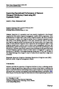
Visualization of Operational Performance of Grid-Connected ... - MDPI
Recommend Documents
Jan 16, 2018 - Pump System Utilizing Recycled Water as Heat Sink ..... the heating outputs and the OA temperature were derived with a curve-fit regression.
Jun 4, 2013 - large volumes of multi-sourced data using open-source software for the ... Complexity and background noise in remote sensing signatures from open ... elevation-sensitive interpolation of climate station data and digital ...
Dec 1, 2017 - able Indoor Air Quality is also maintained (using metabolic CO2 as indicator) and (c) energy costs are .... the system indicating the location of the sensors used to control .... CO2. Telaire 7001. 0 to 2500 ppm. ±50 ppm or 5% of readi
Washington Luiz Km 235, Zip code 13565-905, São Carlos, São Paulo, Brasil. ... discuss the two principal themes on the subject: Operational Strategy and ...
Franco phonic ergonomics) to which they are subjected (6). See Table 1. Table 1 â Points of view of the different actors in the company. Social Agent. Interests.
Dec 31, 2013 - efficiency and service will have the prime responsibility of railway. .... These procedures can be manual steps or an automated cascade. ...... In case of any emergency, accident or natural calamity like flood, cyclone etc., a second .
Aug 1, 2017 - University of Cambridge. The notionally high-performance office/laboratory building implemented two voluntary design frameworks during ...
Apr 14, 2016 - Systems Measured by EntropyâCase Studies ... From a management science point of view, a supplier-customer system belongs to the broad.
Jul 20, 2016 - search for clean and sustainable energy resources [1â3]. ... periods of time without any light using diverse substrates such as organic wastes.
emissions. 1 Introduction. According to Society of Automotive Engineers, an hybrid vehicle is âa vehicle with two or more energy storage systems both of which ...
Things (IoT) in Indonesia Telecomunication Company ... helpdesk, technical dashboard â application layer, technical dashboard â connectivity layer, customer.
More recently, an operational automatic pixel-based near-real- time four-band .... availability of adequate reference (training/testing) data sets derived from field ..... the lever: Give me a place to stand on, and I will move the Earth. ...... Dec.
Oct 12, 2015 - Abstract: Fundamental changes concerning the development of photovoltaic (PV) installations in the Czech Republic (CR) have occurred after ...
vations with the Canadian Meteorological Center. (CMC) Global Environmental ... tem, which we shall call the University of Washington. EnKF (UW EnKF), is ...... commercial airlines: American, Delta, Federal Express,. Northwest, United, and ...
Waddock, S. A. & Isabela, L. A. (1989). Strategy, beliefs about the environment, and performance in a banking simulation. Journal of Management, 15(4), 617â.
Jan 28, 2010 - modernization of Upper Swat Canal (USC) irrigation system, the water allowance ... hydraulic model·Irrigation management transfer.
May 20, 2015 - source praising a friend written by Samuel T. Coleridge in 1816 [1]. From its first record to present, technological and social progress have ...
Texas Transportation Institute (TTI) and Parsons Brinckerhoff Inc.. New Jersey I-80 and. 5. I-287 HOV Lane Case Study. Final Report for FHWA, Jul 2000. 6. 7.
ity of MRP-II in the Semi-Process Industry, Van Gorcum, Assen, The Nether- lands. VAN WEZEL, W. (2001), .... De correlaties kunnen op twee vlakken bestaan:.
A Garmin VIRB-XE camera registered the pictures and videos for each test run ... Part Alignment, RAS-L-1, In Guide for the Design of Rural Highways, Road and ...
to experience a wide range of dust and sand particles during operation. Unclogged Filter Performance. The performance of a clean filter is dependent upon its.
Jul 5, 2016 - Data Visualization Approach for Operational Loading Variations of an. Aircraft Wing Box using Vibration based Damage Detection. Sharafiz A.
Figure 5: HF I/O Time Tunnel View. Figure 6 shows time tunnel end views of in- put/output activity for the QCRD code. Both hard- ware con gurations show a ...
Visualization of Operational Performance of Grid-Connected ... - MDPI
May 23, 2018 - to calculate the total irradiation in the plane of array on an hourly basis. ..... information to individuals or policy-makers to make informed ...
energies Article
Visualization of Operational Performance of Grid-Connected PV Systems in Selected European Countries Bala Bhavya Kausika *, Panagiotis Moraitis
Received: 20 April 2018; Accepted: 21 May 2018; Published: 23 May 2018
Abstract: This paper presents the results of the analyses of operational performance of small-sized residential PV systems, connected to the grid, in The Netherlands and some other European countries over three consecutive years. Web scraping techniques were employed to collect detailed yield data at high time resolution (5–15 min) from a large number (31,844) of systems with 741 MWp of total capacity, delivering data continuously for at least one year. Annual system yield data was compared from small and medium-sized installations. Cartography and spatial analysis techniques in a geographic information system (GIS) were used to visualize yield and performance ratio, which greatly facilitates the assessment of performance for geographically scattered systems. Variations in yield and performance ratios over the years were observed with higher values in 2015 due to higher irradiation values. The potential of specific yield and performance maps lies in the updating of monitoring databases, quality control of data, and availability of irradiation data. The automatic generation of performance maps could be a trend in future mapping. Keywords: performance ratio; annual yield; GIS; PV system; spatial analyses
1. Introduction Recent years have seen a constant growth in solar photovoltaic technology (PV). Several countries have utilized this potential to create a competitive market in view of a green energy future, which led to an increase in small and medium-sized residential solar PV installations [1,2]. These small-sized installations (with capacities less than 10 kWp) are scattered and operate under diverse conditions without adequate monitoring equipment. Studies show that most of these systems perform adequately, but due to a lack of systematic data collection, performance validation was mainly focused on specific geographic areas with a limited amount of systems [3,4]. A “Photovoltaic Geographical Information System” (PVGIS) system was designed to provide performance assessments to an accuracy that is suitable for small installations and for estimating the potential solar energy over large regions at any location in Europe [5]. Although this large-scale GIS (Geographic Information System) database of solar radiation and ambient temperature has been created to estimate energy output from crystalline silicon PV systems and solar water heating systems, it does not provide continuous monitoring or performance evaluation for small-sized, grid-connected PV systems. Currently available monitoring technology in the market is capable of providing owners with sophisticated web tools to monitor their production and system performance at any point during the day, besides measuring energy production. With the advent of such hardware and smart-metering
Energies 2018, 11, 1330; doi:10.3390/en11061330
www.mdpi.com/journal/energies
Energies 2018, 11, 1330
2 of 10
technology, high-resolution monitoring data is publicly available, which is uploaded daily on web platforms, however, in some cases only owners can view this data. With the huge amount of data that is available due to the monitoring equipment, abnormalities can be compared with additional data (remote sensing imagery) for identification of reasons for underperformance or fault detections [6]. Monitoring small grid-connected PV systems to minimize financial losses has also been explored [7] along with the need for long-term monitoring for reliability and increased PV performance [4]. In [1,8], the authors show the importance of using a graphical supported analysis of monitoring and operation of PV installations for fault detections. In our earlier work [9,10], we show how technical aspects and geographical location of PV systems affect PV performance. In this paper, geographic information systems (GIS) are employed to analyze, visualize, and map PV monitoring data from five countries, namely, The Netherlands, France, Germany, Belgium, and Italy. We also present and discuss methods for visualization and detection of underperforming or overperforming systems for further analysis, performance ratio analysis of systems, and spatio-temporal mapping of performance differences. 2. Method Data used for the analyses was collected using online services provided by Solar Log [11] and SMA [12], which also ensured data legitimacy. Solar Log has users over a hundred countries and is one of the major key players in monitoring applications, though it has lost a lot of its clients after 2015. SMA is one of the specialists in photovoltaic inverter system technology. The code used in this research was developed to extract online data and was designed using Python programming [13]. The objective of the web scraping code was to mimic human navigation through web pages of SMA and Solar Log, and to locate and save information that was available to the user [9]. This means that the monitoring information pages of different PV systems was retrieved and saved accordingly. This information was later organized into datasheets. In this way, high temporal resolution yield data (5 min) and other system metadata like orientation, tilt, type of module, etc. were obtained. Recently, privacy constraints have been put on the data, and these data are not available publicly anymore. In total, data from about 31,844 systems were collected for the years 2012–2016 from 5 different countries in Europe, namely, The Netherlands, France, Germany, Belgium, and Italy. In order to calculate the performance ratio (PR) of all the systems, system yield and reference yield are required. System yield is obtained from the data collected by web scraping and reference yield is calculated using the Olmo model [14]. This model requires irradiation data [15]. Hourly global horizontal irradiation data obtained from the 31 ground-based stations of the Royal Netherlands Meteorological Institute (KNMI) were used to compute the reference yield for The Netherlands. These stations cover the entire country. For each installation in the database, irradiation data was collected by linking it to the closest ground station, in order to minimize the uncertainties in the irradiation data. Note that no system was further away than ~30 km from the nearest KNMI station. The tilt and orientation for every system has also been obtained from web-scraped data of PV systems. The Olmo model was then used to calculate the total irradiation in the plane of array on an hourly basis. This study does not take into account effects such as shading as the aim of the paper is to visualize performance rather than detect reasons behind over- or underperformance [16]. The PR was calculated using Equation (1), where Yf is the final system yield and Yr is the reference yield [15]. Since high-resolution, up-to-date annual irradiation data was not available for the rest of the countries, PR was calculated only for The Netherlands. PR =
Yf Yr
(1)
Geographic Information System (GIS) is a “powerful set of tools for collecting, storing, retrieving at will, transforming, and displaying spatial data from the real world” [17]. Based on the principles of geography, cartography, etc., GIS is used for integration of different data types. It is a very powerful tool when it comes to analyses of spatial information, layering or organizing layers of information into
Energies 2018, 11, 1330
3 of 10
Energies 2018, 11, x FOR PEER REVIEW
3 of 10
visualizations using maps and 3D scenes [18]. There are several GIS software packages available in packages available in the market but ArcGIS [19]tool is afor leading licensed tool forgeo-analyses, performing the market today, but ArcGIS [19]today, is a leading licensed performing powerful powerful which will in this paper as an example tool. which willgeo-analyses, be used in this paper as be anused example tool. Visualizations Visualizations of of the the performance performance ratio, ratio, the the locations locations of of the the installations, installations, and and yield yield and and performance performance maps maps were were created created using using the ArcGIS platform. An An inverse inverse distance distance weighted weighted (IDW) (IDW) interpolation interpolation technique technique was was used used to to create create the the performance performance ratio ratio maps maps and and specific specific yield yield maps maps for for different years of ofdata datacollection. collection.Although Although data from around 31,800 systems available (2012– different years data from around 31,800 systems was was available (2012–2016), 2016), only those systems that recorded data continuously for three consecutive (between only those systems that recorded data continuously for three consecutive yearsyears (between 20142014 and and 2016) to compare differences in yield generation. This provides understanding 2016) werewere usedused to compare the the differences in yield generation. This provides an an understanding of of how system performance varies spatially (over geographic areas) and helps identifying outliers how system performance varies spatially (over geographic areas) and helps in in identifying outliers in in data. additiontotobeing beingable abletotovisualize visualizethe theresults, results,looking looking into into the diffusion of distributed thethe data. InInaddition distributed systems systems within within aa country country or or area area allows allows for for the the computation computation of of geo-statistics geo-statistics pertaining pertaining to to the the region region which which are useful for policy implementation. 3. Results Results and and Discussion Discussion 3. From 2011 2011 to to 2016, 2016, data data from from more more than than 31,800 31,800 systems systems was was collected collected and and analyzed. analyzed. However, However, From only 7894 7894ofofthem themwere wereconsistently consistently delivering valid data more 350 days per year at only delivering valid data for for more thanthan 350 days per year for atfor least least three consecutive (2014–2016). The capacity total capacity of these systems was about 102 MWp three consecutive years years (2014–2016). The total of these systems was about 102 MWp with withof56% ofhaving them having lower capacity than and 10 kWp being than kWp 56% them a loweracapacity than 10 kWp only and 1.1%only being1.1% larger thanlarger 50 kWp (see50 Figure (seeThe Figure 1). value The mean was The 12 kWp. Thedistribution spatial distribution of all the installations with system 1). mean wasvalue 12 kWp. spatial of all the installations with system size size information is illustrated in Figure 2. The variation in average composition of the systems information is illustrated in Figure 2. The variation in average sizesize andand composition of the systems in in each country is a direct reflection of the country’s policies on PV subsidy schemes. each country is a direct reflection of the country’s policies on PV subsidy schemes.
Figure Figure 1. 1. System System size size distribution distributionof ofsystems systemswith withcapacity capacityof ofless lessthan than100 100kWp kWpfor forfive fivecountries. countries. The The red red line illustrates the mean value of 12 kWp.
A high concentration of small-scale domestic installations is observed in Germany, Belgium, and A high concentration of small-scale domestic installations is observed in Germany, Belgium, the Netherlands with 64% of the systems in Germany. The Netherlands and Belgium have most of and The Netherlands with 64% of the systems in Germany. The Netherlands and Belgium have most the systems’ total capacity under 5 kWp. While in Germany only 7.2% of the installations fall in this of the systems’ total capacity under 5 kWp. While in Germany only 7.2% of the installations fall in category, 45% of the PV of the systems installed are still below 10 kWp. Though the monitoring this category, 45% of the PV of the systems installed are still below 10 kWp. Though the monitoring procedure might have started at a later time, most of the systems from the sample were installed procedure might have started at a later time, most of the systems from the sample were installed between 2008 and 2014. between 2008 and 2014. Figure 2 shows the location of each PV system, categorized by system capacity. Data collected Figure 2 shows the location of each PV system, categorized by system capacity. Data collected from from the monitoring systems and organized in a database was imported into GIS to create this map. the monitoring systems and organized in a database was imported into GIS to create this map. Clearly, Clearly, large numbers of systems are concentrated in Germany, Belgium, and the Netherlands. Some large numbers of systems are concentrated in Germany, Belgium, and The Netherlands. Some of the of the systems had faulty location information and hence were not included in the map. Most of the systems are also concentrated in the North where irradiation is lower, rather than in the South where there is higher irradiation.
Energies 2018, 11, 1330
4 of 10
systems had faulty location information and hence were not included in the map. Most of the systems are also concentrated in the North where irradiation is lower, rather than in the South where there is higher 2018, irradiation. Energies 11, x FOR PEER REVIEW 4 of 10
Figure 2. Spatial distribution of the data sample for the Netherlands, Belgium, France, Germany, and Italy. Figure 2. Spatial distribution of the data sample for The Netherlands, Belgium, France, Germany, and Italy.
3.1. Yield Analysis and Performance Ratio
3.1. Yield Analysis and Performance The available data was foundRatio to be varying through different time periods as new installations were added every year. Also, not all the systems recorded data for all the years. Therefore, only those The available data was found to be varying through different time periods as new installations systems that had been consistently delivering data for the three consecutive years (2014–2016) have were added every year. Also, not all the systems recorded data for all the years. Therefore, only those been considered for analysis. Furthermore, since the interest is in monitoring small-scale installations, systems that had been consistently delivering data for the three consecutive years (2014–2016) have annual yield analysis of systems below 20 kWp for the years 2014–2016 has been conducted for the been considered for analysis. Furthermore, since the interest is in monitoring small-scale installations, Netherlands, France, Germany, Belgium, and Italy. These countries were found to have the highest annual yield analysis of systems below 20 kWp for the years 2014–2016 has been conducted for amount of data records from the data collection. The Netherlands, France, Germany, Belgium, and Italy. These countries were found to have the highest The mean value and the standard deviation of the performance of systems of each sample is amount of data records from the data collection. shown in Figure 3: here we show the annual specific yield, i.e., generated amount of energy divided The mean value and the standard deviation of the performance of systems of each sample is by system capacity (kWh/kWp). These are known to be affected by a number of environmental and shown in Figure 3: here we show the annual specific yield, i.e., generated amount of energy divided operational factors [20]. Moreover, a wider spread of yearly yield values can be expected from by system capacity (kWh/kWp). These are known to be affected by a number of environmental countries covering larger areas as a result of the variation of irradiation levels at different latitudes. and operational factors [20]. Moreover, a wider spread of yearly yield values can be expected from The distribution of annual system yield for the Netherlands, Belgium, Germany, and Italy is shown countries covering larger areas as a result of the variation of irradiation levels at different latitudes. in Figure 4. France has only 95 installations between 2014 and 2016 out of which 76 systems are below The distribution of annual system yield for The Netherlands, Belgium, Germany, and Italy is shown in 20 kWp capacity, while Germany has nearly 3900 systems, and Belgium 1700. Therefore, France has Figure 4. France has only 95 installations between 2014 and 2016 out of which 76 systems are below higher mean yields and only four outliers due to sample size. Between 2014 and 2016, the annual 20 kWp capacity, while Germany has nearly 3900 systems, and Belgium 1700. Therefore, France has yield increased in 2015. However, the decrease or increase in yields falls within standard deviations, higher mean yields and only four outliers due to sample size. Between 2014 and 2016, the annual yield but at the same time relates directly to the decrease or increase in solar irradiation on a country level. increased in 2015. However, the decrease or increase in yields falls within standard deviations, but at Performance ratio (PR) analysis was conducted for the Netherlands which revealed a mean PR the same time relates directly to the decrease or increase in solar irradiation on a country level. value of 79% for the year 2016 and 80% for 2014 and 2015. The PR values were calculated with an Performance ratio (PR) analysis was conducted for The Netherlands which revealed a mean PR average daily PR value over a year. These values are close to the results of an earlier study performed value of 79% for the year 2016 and 80% for 2014 and 2015. The PR values were calculated with an in Germany [21]. The sample size for this estimation was about 600 installations. The number of PV average daily PR value over a year. These values are close to the results of an earlier study performed installations in the Netherlands significantly increased from 2009, but their performance dropped in in Germany [21]. The sample size for this estimation was about 600 installations. The number of PV 2016 in comparison to 2014 (Figure 5). Systems installed in 2013 performed well in 2014 and 2015, installations in The Netherlands significantly increased from 2009, but their performance dropped while in 2016, a lot of outliers were observed. In some cases, the large variation in PR values could also be due to technical errors in data collection.
Energies 2018, 11, 1330
5 of 10
in 2016 in comparison to 2014 (Figure 5). Systems installed in 2013 performed well in 2014 and 2015, while in 2016, a lot of outliers were observed. In some cases, the large variation in PR values could also Energies 11, x FOR PEER 5 of 10 be due2018, to technical errorsREVIEW in data collection. Energies 2018, 11, x FOR PEER REVIEW
5 of 10
Figure 3. Distribution of specific yield by country from 2014 to 2016 for systems less than 20 kWp. Figure Distribution of yield by from 2014 to for systems less 20 kWp. Figure 3.3. Distribution of specific specific yieldwith by country country from 2014the to 2016 2016 for mean, systems less than than kWp. Highest yields were recorded in 2015, Italy (IT) having highest followed by20 France Highest yields were recorded in in 2015, with Italy (IT)(IT) having the highest mean, followed by France (FR), Highest yields were recorded 2015, with Italy having the highest mean, followed by France (FR), Germany (GER), Belgium (BE), and the Netherlands (NL), respectively. Germany (GER), Belgium (BE), and The Netherlands (NL), respectively. (FR), Germany (GER), Belgium (BE), and the Netherlands (NL), respectively.
Figure 4. Distribution of specific yield for the year 2016 for Italy, Germany, Belgium, and the Netherlands. Figure 4. 4. Distribution of specific specific yield yield for for the the year year 2016 2016 for for Italy, Italy,Germany, Germany,Belgium, Belgium,and andThe the Netherlands. Netherlands. Figure Distribution of
Energies 2018, 11, 1330 Energies 2018, 11, x FOR PEER REVIEW
6 of 10 6 of 10
Figure Distribution of ofperformance performanceratio ratioofof theNetherlands Netherlands between 2014 for systems Figure 5. 5. Distribution The between 2014 andand 20162016 for systems that that have been installed from 2009 to 2013. have been installed from 2009 to 2013.
3.2. Geographical Variation of Specific Yield 3.2. Geographical Variation of Specific Yield Point data (vector information) collected from the web monitoring services has been converted Point data (vector information) collected from the web monitoring services has been converted to to images (raster information) by using interpolation techniques. Interpolated data is visualized using images (raster information) by using interpolation techniques. Interpolated data is visualized using color scales stretched using specific bins of annual yield values. From these images/maps, outliers color scales stretched using specific bins of annual yield values. From these images/maps, outliers can be quickly discerned to locate PV systems with minimum or maximum yields, thus providing a can be quickly discerned to locate PV systems with minimum or maximum yields, thus providing starting point for further analyses into the reason behind the system’s under- or overperformance. a starting point for further analyses into the reason behind the system’s under- or overperformance. The maps can be compared to the country irradiance maps to check for irradiation trends in the The maps can be compared to the country irradiance maps to check for irradiation trends in the particular year, as yield values are related to irradiation values. This provides a quick approximation particular year, as yield values are related to irradiation values. This provides a quick approximation of the variation of performance over the country. of the variation of performance over the country. Figure 6 shows an interpolated map of annual yield of the Netherlands and Italy for three years Figure 6 shows an interpolated map of annual yield of The Netherlands and Italy for three years with dots representing the location of the systems. Inverse Distance Weighted (IDW) interpolation with dots representing the location of the systems. Inverse Distance Weighted (IDW) interpolation technique was used to generate the maps. Higher yield values have warmer and darker shades (reds) technique was used to generate the maps. Higher yield values have warmer and darker shades (reds) and lower yield values have a blue shade. A variation in yield values is observed within the countries, and lower yield values have a blue shade. A variation in yield values is observed within the countries, while it should be noted that these variations can further be optimized using different color scales while it should be noted that these variations can further be optimized using different color scales and and data stretching methods. A few examples of this are shown below. data stretching methods. A few examples of this are shown below. Although variations over the years are not very prominent because of the type of stretch used Although variations over the years are not very prominent because of the type of stretch used for for data visualization and the data sample (system size up to 20 kWp), it could still be distinguished data visualization and the data sample (system size up to 20 kWp), it could still be distinguished that that 2015 has higher annual yields. A min–max stretch was used to visualize data with the same scale 2015 has higher annual yields. A min–max stretch was used to visualize data with the same scale of of minimum and maximum values for the three years to maintain consistency. minimum and maximum values for the three years to maintain consistency. When using a different data stretching method (see, for example, Figure 7a), extreme deviations When using a different data stretching method (see, for example, Figure 7a), extreme deviations in in data (bright spots) can be identified around systems with extreme yield values. These extreme data (bright spots) can be identified around systems with extreme yield values. These extreme values values carry a higher weight factor during interpolation causing the spot or bleeding effect. As carry a higher weight factor during interpolation causing the spot or bleeding effect. As mentioned mentioned earlier, these spots can be separated out as outliers or as inadequately performing systems. earlier, these spots can be separated out as outliers or as inadequately performing systems. Moreover, Moreover, if high resolution irradiation data is available, the database of collected information could if high resolution irradiation data is available, the database of collected information could be explored be explored by irradiation zones in addition to spatial diffusion or technical criteria. by irradiation zones in addition to spatial diffusion or technical criteria. An example of different stretching techniques is shown in Figure 7, in which two types of data An example of different stretching techniques is shown in Figure 7, in which two types of data stretching were used over a color scale. In Figure 7a, a percentage clip method was used, where the stretching were used over a color scale. In Figure 7a, a percentage clip method was used, where the values values displayed are cut-off percentages of highest and lowest values, while Figure 7b displays values displayed are cut-off percentages of highest and lowest values, while Figure 7b displays values between between the actual or set minimum and maximum. A smoothing effect can also be seen in Figure 7b, the actual or set minimum and maximum. A smoothing effect can also be seen in Figure 7b, while it is while it is easier to pick out underperforming or overperforming systems to analyze them further easier to pick out underperforming or overperforming systems to analyze them further from Figure 7a. from Figure 7a.
Energies 2018, 11, 1330
7 of 10
Energies 2018, 11, x FOR PEER REVIEW
7 of 10
Energies 2018, 11, x FOR PEER REVIEW
7 of 10
Figure 6. Annual specific yield variation from the installations (up to 20 kWp) in the Netherlands Figure 6. 6. Annual variation from installations (up to 20 20 kWp) kWp)techniques. inthe TheNetherlands Netherlands Figure Annual specificyield yield variation from the thevisualized installations (up to in (above) and Italyspecific (below) for the years 2014–2016, using interpolation (above) and Italy (below) for the years 2014–2016, visualized using interpolation techniques. (above) and Italy (below) for the years 2014–2016, visualized using interpolation techniques.
Figure 7. Annual specific yield variation from the installations (up to 20 kWp) for Belgium visualized Figure 7. Annual specific yield variation from the installations (up Belgium using different typesyield of data stretching forthe 2016. Data stretching techniques (a) percentvisualized clip and Figure 7.two Annual specific variation from installations (upto to20 20kWp) kWp)for for Belgium visualized using two different types datastretching stretchingfor for 2016. 2016. Data Data stretching clip and (b) min-max used for data visualization. using two different types ofof data stretchingtechniques techniques(a)(a)percent percent clip and (b) min-max used for data visualization. (b) min-max used for data visualization.
Another example of the power of GIS in visualization is shown in Figure 8, where the mean Another example of the power of GISthresholds in visualization is shown Figure 8, The where the mean specific yield for Germany using different of system sizes isinpresented. variation in Another example of the power of is GIS in visualization is shown in Figure 8,The where the mean specific yield forsystems Germany different thresholds of system sizestoiswhen presented. variation in specific yield of up using to 20 kWp much smoother compared only systems up to 10 specific yield forofGermany using thresholds of system sizes presented. The variation specific yield systems up to 20different kWp is much compared toiswhen only systems up to 10 in kWp are considered. For example, the systems in smoother the highlighted area (red box in both images) shows specific yield of systems up to 20 kWp much compared to when only up to 10 kWp kWp are considered. For example, theissystems in the highlighted (red in systems both images) shows underproduction when compared with largersmoother systems (