Feature Article
Visualization of Structured Nonuniform Grids O
perational forecasters and weather researchers need accurate visualization of atmospheric data from both computational models and observed data. Although these two applications share some requirements, they have different needs and goals. Atmospheric phenomena are visualized at various scales and on a wide variety of grids, so weather visualization packages must have flexible sampling systems. Tools that can handle a wide variety of grids let researchers apply many powerful techniques within atmospheric research, such as simulation and measurement data comparisons and multiple model analysis. Researchers often choose meteorological grid structures based on efficient computation or limitations of the measurement system, complicating the mapping from the Cartesian rendering space to the data’s A texture-based volume computational space. Although uniform grids form the rendering architecture for basis for a wide variety of applications and are comparatively easy to nonuniform meshes avoids sample, many applications, including fluid dynamics simulations, resampling errors while weather models, ocean models, and Doppler measurement, use nonuniretaining the original grid’s form, structured grids that provide higher sampling densities in areas of structure. greater variation, interest, and accuracy. Unfortunately, these nonuniform grid structures are more difficult to manage in texture-based volumerendering applications (see the “Previous Work in Visualizing Nonuniform Grids” sidebar for other work in this area). Although we can resample the data to a uniform grid, this method often introduces grid artifacts not present in the original data, and can require significantly more storage. The grid should also be as small as possible so the relevant data fields can fit into the graphics processing unit (GPU) memory. We’ve developed a visualization tool for atmospheric science researchers and research weather forecasters that allows the 3D visualization of measured radar data and rendered numerical model data to show the 3D structures as well as how the weather event would look when observed in the field. Our system lets us load the original data directly onto the graphics hardware, with the grid mapping from the rendering space to the grid
46
January/February 2006
Kirk Riley, Yuyan Song, Martin Kraus, and David S. Ebert Purdue University Jason J. Levit National Oceanic and Atmospheric Administration
space programmed on the GPU. This method is flexible enough to handle the grids important in meteorological research and enables the application of advanced visualization methods available in texture-based slicing systems. The visually accurate rendering of weather data can be useful for training weather spotters, evaluating forecasting models, training forecasters to interpret radar data, and comparing sensor data to observed weather events.
Texture-based volume-slicing rendering Since volume rendering’s introduction in 1988, it has been an essential 3D visualization tool. Applying modern graphics hardware to the volume-rendering problem has allowed for complex pixel computation and advanced lighting models1 in interactive volume visualization. Essentially, modern graphics hardware lets us program complex per-pixel fragment programs. For texture-based volume-rendering algorithms, the software usually stores the volume data in a hardware 3D texture and generates a set of sampling or slicing planes to sample the data. Most implementations use eye-aligned planes, meaning that the slicing plane normal is along the ray from the eye to the volume’s center. We can generate these planes in front-to-back or back-to-front order with respect to the eye. When rasterized, each plane samples the volume data at the appropriate location. We then apply a transfer function (either through a dependent texture read or in a fragment program function) that maps the data to the appropriate color and opacity at that point in space. It blends this color with the previous samples to calculate the contribution to the eye. Let Ci+1(u) be the next pixel color value at the rasterized pixel coordinate u, Ci(u) be the current value in the buffer, and Cs be the color calculated for the current sample on the slicing plane. Also, let αi+1(u) be the new opacity value at u, αi(u) be the pixel’s current opacity, and αs be the current sample’s opacity. For front-to-back rendering, we perform compositing according to Equation 1. Ci+1( u ) = Ci ( u ) + (1 − α i ( u ))α sC s α i+1( u ) = α i ( u ) + (1 − α i ( u ))α s
(1)
For back-to-front rendering, we accomplish compositing using Equation 2.
Published by the IEEE Computer Society
0272-1716/06/$20.00 © 2006 IEEE
Previous Work in Visualizing Nonuniform Grids
or iterative search methods such as stencil walking.8
We can apply many techniques to the visualization of nonuniform grids. Software techniques have focused on the general problem of transforming between the physical and computational spaces.1,2 Some of these software systems include powerful operational forecasting systems3 but are less suited for the interactive and flexible exploration of research data. We can render complex grids through raycasting of tetrahedral meshes.4 Projected tetrahedra and methods allow hardwareaccelerated rendering of nonuniform structured and unstructured grids.5 Visibility ordering is an essential aspect of these methods.6 Splatting systems are particularly well suited to unstructured data, but abandon the cell-connectivity available in nonuniform structured grids. Neither of these methods are well suited for the self-shadowing rendering techniques we wish to apply, because we have two distinct viewpoints— one from the eye and one from the light source. Although these algorithms can handle a wider range of grids than our approach, our system introduces an efficient sampling method for advanced lighting and transfer function on graphics hardware without needing visibility sorting. Our framework for visualizing data on functionally encoded grids lets us perform sampling in programmable graphics hardware at the pixel level, without requiring revoxelization7
Ci+1( u ) = (1 − α s )Ci ( u ) + α sC s
(2)
References 1. R.B. Haber, B. Lucas, and N. Collins, “A Data Model for Scientific Visualization with Provisions for Regular and Irregular Grids,” Proc. IEEE Visualization, IEEE CS Press, 1991, pp. 298-305. 2. L.A. Treinish, “A Function-Based Data Model for Visualization,” Proc. IEEE Visualization, Late Breaking Hot Topics, IEEE CS Press, 1999, pp. 73-76. 3. L.A. Treinish, “Task-Specific Visualization Design,” IEEE Computer Graphics and Applications, vol. 19, no. 5, 1999, pp. 72-77. 4. M. Weiler et al., “Hardware-Based Ray Casting for Tetrahedral Meshes,” Proc. IEEE Visualization, IEEE CS Press, 2003, pp. 333-340. 5. P. Shirley and A. Tuchman, “A Polygonal Approximation to Direct Scalar Volume Rendering,” Proc. 1990 Workshop Volume Visualization, vol. 24, no. 5, ACM Press, 1990, pp. 63-70. 6. N. Max et al., “Volume Rendering for Curvilinear and Unstructured Grids,” Computer Graphics Int’l, 2003, p. 210. 7. J. Leven et al., “Interactive Visualization of Unstructured Grids Using Hierarchical 3D Textures,” Proc. 2002 IEEE Symp. Volume Visualization and Graphics, IEEE Press, pp. 37-44. 8. P. Buning, “Numerical Algorithms in CFD Post-Processing,” Computer Graphics and Flow Visualization in Computational Fluid Dynamics, von Karman Inst. for Fluid Dynamics Lecture Series, 1989.
sible if the eye and light are collinear, we consider the two cases in Figure 1. When the angle between the eye and light is acute, the slice normal is halfway between the eye and light vectors. When the angle is obtuse, the slice normal is halfway between the inverted light vector and the eye vector. Next, for each sample, we calculate the contribution to the eye (or frame) buffer using the light buffer’s cur-
Opacity accumulation is irrelevant for back-to-front rendering, so we rarely store it. Volumetric lighting provides many important spatial cues but can be extremely complex to compute in the presence of multiple scattering. To extend the basic texture-based methods to handle lighting computations, we implemented a half-angle slicing system.1 For efficiency, we designed the lightLight buffer ing approximation to make a single slicing Light buffer pass through the volume. This system renSlicing Slicing plane ders each slice both to the eye buffer, plane Data volume which stores the image, and to a light buffer, which stores the light attenuation Eye buffer Eye buffer from the samples. To track the light attenCi Ci uation accurately, we initialize the light buffer to full intensity, traversing slices in front-to-back order with respect to the light location. It’s important to choose a slicing geomSlicing order Slicing order etry that’s appropriate for both the eye and the light buffers. Ideally, a slice would be (a) (b) normal to both the eye and light directions. Because this slicing geometry is only pos1 Half-angle slicing rendering: (a) acute and (b) obtuse.
IEEE Computer Graphics and Applications
47
Feature Article
rent value and then update the light buffer with the light attenuation calculated on the slicing plane.
Rendering architecture Our system first determines the input data type. The system performs any preprocessing and grid structure approximations the renderer requires for that particular data format. We then store the tables needed for the transfer function and the basis coefficients needed for the grid approximations on the graphics hardware. Floating-point precision controls the quantization error in the textures storing these tables. After we’ve sufficiently characterized the grid, the rendering engine begins. Our rendering engine selects appropriate volume-rendering fragment programs, created with Nvidia’s Cg language in OpenGL. These programs contain the correct mapping from the rendering space to the data space for this particular grid, as we describe in more detail later. (All of the programs use the same rendering code; only the data sampling stage is different.) We then pass all rendering parameters, including gridspecific parameters, to the fragment program. When the preprocessing ends, we begin the rendering loop. Because self-shadowing is essential for understanding the structure of many volumetric data sets, particularly clouds, we use a half-angle slicing lighting model.1 We allocate a single floating-point pixel buffer on the graphics hardware and split it into eye and light halves. Fragment programs initialize the light and eye halves separately. The light fragment program is always the same, but the eye program changes depending on the compositing direction. For front-to-back with respect to the eye, we render the foreground first; otherwise, we first render the background. We then render the sampling slices. We render each slice twice: once to the eye buffer to track the accumulation of light seen on the image plane, and once to the light buffer to track the attenuation of light as it traverses the volume. For each sampling slice in the volume, we select the eye buffer (using a viewport transformation) and enable the appropriate fragment program. At each pixel sample point on the rasterized slice, the program transforms coordinates from the rendering space to the data space and reads the data. It then applies the transfer-function mapping and composites the output color in the pixel buffer according to the appropriate front-to-back or backto-front scheme. Another viewport transformation selects the light buffer, and a light propagation fragment program rasterizes the same slice from the light viewpoint. This program must also perform the appropriate data sampling, transfer function mapping, and composition in the light buffer. When the eye and light fragment programs complete computation in the pixel buffer, the output fragment program writes the final result to the 8-bit-per-channel color frame buffer (further details on the rendering architecture are available elsewhere2). Our transfer function system3 enables realistic rendering, as well as some simple color-based transfer function options implemented on the graphics hardware. Although our sampling approach requires some specific programming for each data set type, conceptually it isn’t more complex than programming a uniform
48
January/February 2006
resampling system. It simply uses the opposite transformation (rendering space to data space, not data space to a Cartesian uniform grid in world space) and performs it at the fragment level, letting us use the original data.
Sampling nonuniform structured grids At its core, our system is an extension of our earlier system.3 To allow nonuniform grid structures, we changed the data model and implemented a per-pixel mapping from the renderer’s physical space to the data’s computational space in the volume-rendering fragment programs. The rendering system transforms between several spaces. Most volume renderers, including ours, model a physical space (p-space), which is a Cartesian system of x, y, z triplets. This space defines the world in which we create the image and is usually analogous to a physical 3D space. We create the data in its own computational space (c-space) based on the simulation or measurement system requirements. The data’s base space (b-space) defines the data elements’ physical location in their own local coordinate system. The mapping from c-space to b-space involves transforming (possibly nonlinearly) the data grid into a local Cartesian coordinate system. The mapping from b-space to p-space must be an affine linear transformation, but b-space is necessary because a single p-space can contain multiple objects, each with its own b-space. For nonuniform structured grids, cell connectivity lets us store the data in texture memory, with adjacent texture elements corresponding to adjacent, if perhaps curved, cells in b- and p-spaces. Our system applies a functional representation of the grid if it’s available; otherwise, it performs a functional approximation of the grid. For a function that is reasonable to evaluate (in constant time) on graphics hardware, this technique produces an O(1) sampling solution. We define a pspace coordinate, p, and a c-space coordinate, c, that serve as a texture index. The transformation from pspace to c-space is Ξ(p), that is c = Ξ(p). For the volume renderer to read the data stored in a 3D texture in the graphics hardware, we program Ξp using fragment programs that map the 3D Cartesian point in p-space to the corresponding point in 3D texture c-space. Therefore, the system performs the transformation per pixel to get the appropriate sampling point in the data grid. Determining the region for which this transformation is valid is also important, particularly if we functionally approximate the grid. Thus, for each pixel, we check bounds to see if the point lies within the data domain. If it does, we calculate the texture coordinate, Ξ(p), and use it to sample the data. For example, consider a 2D scene with two polar data sets, as Figure 2 shows. The c-space dimensions are the radius and azimuth. The b-spaces for these data sets are 2D Cartesian spaces, where the data covers a circular section beginning at the polar origins. The mapping from p-space to b-space (transforming p to p′) for each data set is a simple translation to place the origin at the polar coordinate system origin. The test point pt in Figure 2 is within the b-space coverage of one data set, but not the other. Therefore, we sample only the texture for
p t'
Cy = θ
by
p t"
pt bx
Cx = r
Base space 1
Computational space 1
py p t'
px
2 Twodimensional example of transforming a point, pt, into two data computational spaces (c-spaces).
Cy = θ
by
bx
Cx = r
Base space 2
the data set where the point is within the data domain. For this data set, we calculate the c-space location by the transformation from pt′ to pt′′ = ct. This step completes the overall transformation from p-space to c-space, ct = Ξ2(pt). We use this coordinate to sample the data, and the renderer applies the appropriate transfer function mapping. The Ξ mapping between p-space and c-space presents the largest difference between nonuniform structured grids. For a grid structure with known functionally encoded vertices and a known inverse, this mapping is a simple transformation. If the function is unknown, we must perform an approximation to match the grid vertex locations. One option, which we discuss in detail later, is to perform a polynomial fit of the grid vertices, although any accurate functional approximation that can be implemented on graphics hardware will work.
Applications Two important applications illustrate the implementation process of the data model and architecture. We apply our system to the mass-coordinate grid popular in weather research and forecasting (WRF; see http://wrf-model.org) meteorological simulator data sets, and then describe a method for rendering Doppler data. We then discuss two important aspects of our solutions for these applications: temporal antialiasing and map projections.
Computational space 2 Out of bounds: returns 0
Mass-coordinate data grids Mass-coordinate data grids are common in meteorology, and analogous grids are often used for oceanography data (such as for Naval Research Laboratory layered ocean models). These grids are Cartesian in their lateral dimensions (transverse to the earth plane) and have variable spacing (based on pressure) in the height or depth dimension (normal to the earth plane). Additionally, for meteorological data, these grids follow the underlying terrain. The grids maintain cell connectivity, but the cell spacing in height varies depending on terrain and atmospheric pressure. We applied our system to two WRF data sets. ■ The first is a time-series of the 3 and 4 April 1974 tor-
nado superoutbreak, with the model domain centered over the eastern US, where most of the severe weather occurred. Supercomputers maintained by the Oklahoma Supercomputing Center for Education and Research at the University of Oklahoma generated the simulation. ■ The second simulation is of Hurricane Isabel generated at the National Center for Atmospheric Research. The data grid on both of these mass-coordinate sets is Cartesian in the lateral dimensions (x and z) with a 4,000-meter-per-voxel spacing. The original grid sizes are 349 × 349 × 35 for the tornado outbreak data set, and 500 × 500 × 35 for the Hurricane Isabel data set. For
IEEE Computer Graphics and Applications
49
Feature Article
Metric Peak error Root-mean-square error
Tornado Outbreak
Hurricane
0.013 0.005
0.107 0.028
rendering using a PC graphics card with 256 Mbytes of memory, the user can select a subvolume for visualization with dimensions up to 256 × 256 × 256. Although this partitioning of large data sets common in meteorology is inconvenient, increases in GPU memory will reduce this restriction. We can extend the system to “brick” the data setthat is, decompose it into rectangular sections that fit into texture memoryand render the multiple bricks composing the volume. This mass-coordinate grid stores base and perturbation geopotential values (φb and φp) that determine the grid data height. We define geopotential as the work against the Earth’s gravitational field required to raise a 1-kilogram mass from sea level to the data element’s height. We designed the coordinate system to follow the Earth’s surface, so the lowest height for each data column is essentially a pseudorandom function. We calculate the data’s height in meters by summing these geopotentials and dividing by the acceleration due to gravity. Equation 3 gives the physical height, py (in meters) of a given c-space location, c, for this grid.
()
py c =
() ()
φb c + φ p c
(3)
9.81 meters per second2
This grid is therefore well behaved in the lateral domain but problematic in height. To accommodate the grid, we encode the grid vertices for the height dimension with a polynomial fit. This means we perform one polynomial fit for each lateral grid point (that is, each pair of cx and cz) in the data. Our desired function performs the inverse mapping to Equation 3that is, from height value to index (cy(py)). In the preprocessing
stage, we first normalize the heights by dividing them by the maximum height. We then perform a standard least-mean-square error fit to get the 11 basis coefficients of the 10th-degree polynomial fit. We chose a 10th-degree polynomial because it provides accuracy to within one-eighth of a voxel. We also verifiedby plotting the approximations at several locationsthat the fit doesn’t suffer from unstable artifacts caused by too many coefficients. Table 1 lists the encoding errors for this process. We store the coefficients in the floatingpoint texture (K(px, pz)), indexed by the lateral-dimension texture coordinates, which are also the system’s p-space coordinates. As Equation 4 shows, we denote the basis as B(γpy), where γ contains the scaling factors for converting py to a height in meters, and the division by maximum height normalization. 1 γp y 2 = γp y 3 γp y
( ) ( ) ( )
B γp y
(4)
…
Table 1. Mass-coordinates encoding error in voxels.
Therefore, to calculate the 3D c-space height index, c, from the p-space location, p, we must sample the coefficient texture, evaluate the basis, and perform a dot product. We calculate Ξ(p) using Equation 5. px Ξ p = K px , pz ⋅ B p y pz
()
) ( )
(
(5)
For each pixel sample in the volume-rendering stage, we evaluate the polynomial for the height value using coefficients retrieved from the texture lookup. We use the polynomial’s output as the height-dimension texture coordinate (the lateral dimensions are the same as
0-1 Physical space box
Data computational space Rasterized pixel Rendering in the masscoordinate system.
Data value
(px, py, pz)
3
py Image plane
pz
cy cx K(px, pz)·B(py) = cy
px
cz cx = px
K(px, pz) table px
50
January/February 2006
pz
cz = pz
(a)
(b)
(c)
(d)
4 A slice through the tornado data set rendered with (a) the uncorrected grid, (b) the grid uniformly resampled to 1.8 times its original height, (c) the grid uniformly resampled to 7.3 times its original height, and (d) the grid corrected with our system. for the coefficient lookup) into the original data set. Figure 3 is a diagram of the rendering system for mass coordinates. We also need to perform bounds checking in this process to guarantee that we’re within the data set, because functional fits have unpredictable behavior outside their defined region. Because all of the data columns end at approximately the same height, we perform a p-space check to see if the data is above the data maximum height, discarding it if it is. We check the minimum height by checking for a negative cy. Although the function fit isn’t guaranteed to become negative, in practice the curve goes negative for values below the earth’s surface. Once a sample is rasterized beneath the earth, it has full opacity and we ignore all future samples for that pixel. Figure 4 compares a slice through the tornado outbreak data set rendered without the grid correction and uniformly resampled to 1.8 and 7.3 times the original height dimension, with a slice processed using our sampling technique. Clearly, we must correct the grid for accurate rendering. Additionally, because the application is for accurate atmospheric data rendering, the WRF data type selects foreground and background renderings for handling the volume’s aerial perspective and stores the required parametric data. Therefore, in this application, the lookup table texture contains rendering function tables as well as the basis function coefficient table. Figure 5 shows images of the tornado outbreak data set. We also applied the system to a WRF simulation of Hurricane Isabel, as Figure 6 shows. Our system provides a flexible framework with which meteorologists can explore their research data. The lighting method is field specific, so it provides some intuition as to the data’s components. Meteorologists are trained to inter-
5 Rendering of the tornado outbreak data set: (a) from Earth with aerial perspective, and (b) from the sky without aerial perspective.
(a)
(b)
6 Rendering of the Hurricane Isabel data set, from the sky, without aerial perspective.
IEEE Computer Graphics and Applications
51
Feature Article
7 Doppler radar rendering in Oklahoma during a tornadic storm.
pret physical events based on observations of phenomena. Our rendering method helps them answer, What would this event look like in the sky?—an important question with implications for comparison with real events, as well as for training. Several important events are visible in Figure 5b. The anvil structure on the upper left side of the image is an important region to investigate for severe storm and tornadic activity. These visually familiar renderings of the numerical simulations also provide important visual cues for understanding the weather model data’s components and let the atmospheric scientist’s training help them understand the structures in the data. For example, a cloud researcher immediately identified the absence of medium-scale turbulence in the WRF super cell simulation. A few weeks later, other researchers reported an error in the simulation code that was setting the turbulent kinetic energy to zero. Thus, the renderings can also serve as a visual debugging and validation tool.
Doppler data Another important grid structure for measured weather data is the Doppler radar grid structure. Doppler radar is widely used for weather forecasting and is available online (http://hurricane.ncdc.noaa. gov/pls/plhas/has.dsselect). Whereas most applications focus on 3D Doppler data surface representations, our system samples from the original data grid for direct volume rendering. We applied our system to Nexrad level II WSR-88d Doppler radar data read with a version of the TRMM Radar Software Library (http://trmm-fc. gsfc.nasa.gov/trmm_gv/software/rsl) ported to Windows. This data contains reflectivity, Υ (in decibels z, or dBz), radial wind velocity (in meters per second, or m/s), and spectrum width (a measure of turbulence in m2/s2). Because weather research and training applications need accurate weather data rendering, we’re currently rendering according to visible properties derived from the reflectance field. For atmospheric rendering, determining optical extinction from the reflectivity requires a relationship between the scalar reflectivity and particle concentration (η in 1/m3) of the multiple field. In a preprocess, we apply Ferrier’s calculations4 to determine the mixing ratios (gram of substance per kilogram of air). These calculations give us a method for extracting the mass mixing ratios for rain (Qr), snow (Qs), and hail (Qh) from the single scalar reflectivity value provided by the
52
January/February 2006
Doppler radar output. We interpolate tabulated values from the 1976 US standard atmosphere model5 to calculate the temperature and pressure this model requires, or use measured data from weather balloons for improved accuracy. Next, we calculate the particle concentration—η(1/m3)—and extinction coefficient as described elsewhere.3 Finally, we store this extinction coefficient in the volume texture. The radar station takes points in roughly even intervals in polar coordinates. The c-space is thus a rectilinear space in radius (r = cx), azimuth (φ = cy), and altitude (θ = cz). The interval for the radial coordinate is approximately 1 kilometer and the interval for φ is 1 degree. Depending on weather conditions, a Doppler station samples in one of four scan modes—or volume coverage patterns (VCPs)—that determine the interval for θ, which ranges from 0 degrees to anywhere between 4.5 and 19.5 degrees, depending on the VCP mode. VCP 31 and 32, the simplest and most common modes, have a linear 0.97-degree separation between cells. More complex modes, such as VCP 11 and VCP 21, have a more complex θ function. In this work, we use a fifth-degree polynomial basis approximation for this nonlinear function, with a peak error of 0.082 voxels and a root-meansquare (RMS) error of 0.042. We chose this order as a good trade-off between the solution’s accuracy and stability. Let the basis coefficients for the given scan mode be Λ. Because we normalize physical and computational space coordinates to [0-1], the transformation from p-space to c-space becomes cx = 2K x
( p − 0.5) + ( p
) (
)
2
2
x
y
− 0.5 + pz − 0.5
p − 0.5 c y = K y arcttan z p − 0.5 x p y − 0.5 θn = K z arctan 2 px − 0.5 + pz − 0.5
(
(
c z = Λ ⋅ 1,θn ,θ2n ,...,θ5n
)
) (
)
2
2
We test the range of the applied arctan function. The φ function ranges from 0 to 360 degrees. Because boundaries on θ depend on the radar station’s sweep mode, we determine the boundary checking using a set of runtime parameters. Minimum θ (not normalized to 0-1 like θn) is 0 degrees; its maximum is between 5 and 15 degrees, depending on the sweep mode. We typically limit the radius r to be between 0 and 460 km. Figure 7 is a Doppler image taken around the time of the 3 May 1999 Oklahoma City tornado. The storm cell has the characteristic anvil-like shape indicating possible tornadic activity. Figure 8 shows a Doppler image of Hurricane Ivan over Alabama on 16 September 2004. The circular structure in the center of the image’s top half doesn’t show the hurricane’s eye, but is an artifact of the Doppler radar’s data coverage. Figure 9 compares our sampling technique (Figure 9a), uniform resampling of the grid to twice the original
size (Figure 9b), and uniform resampling of the grid to the same size (Figure 9c). Our system lets scientists partition the reflectivity data into various fields and manipulate their combination for an accurate view of the weather event. This technique has important implications for the comparison of multiple models and representations, and helps users understand how the different sources represent a given meteorological event. Our system also has important applications in training and education, because these multiple sources can be visualized similarly to field observation.
8 Rendering of Hurricane Ivan from an aerial viewpoint.
Temporal antialiasing Doppler data suffers from some well-known timealiasing phenomena. Performing a sweep takes several minutes, and thus by the time the radar system takes the later samples, the measured event might have shifted, producing results that can be misleading. Fortunately, Doppler radar systems take samples consecutively. We can exploit this fact to remove some temporal effects. Nexrad level II data contains timestamp information for each sweep. We can use this information to better approximate the data values at a given reference time. Consider two consecutive radar sweeps. We want to find the data at a given reference time Tr, which will be the beginning of the second sweep. For each sample point s in space, there is a datum value from each of these data setsDi(s) and Di+1(s). Each sample location also has a time valueTi(s) and Ti+1(s). We base the interpolation parameter, σ(s), on the distance in time from the reference location:
()
σs =
gitude coordinates. We then transform the coordinates to a Cartesian space, and finally perform the previously described mapping from Cartesian to the Doppler or WRF grid. We’ve implemented the capability for meteorologists to use the Lambert conformal projection, an angle-preserving projection; other projections would follow similarly. Lambert conformal projection requires two standard latitudes: φ1 and φ2. Equation 7 gives the mapping from the original lateral map coordinates in the Lambert system (lx, ly) to latitude and longitude world coordinates, (px, py).6 F π px = 2 arctan 1 n − ρ 2 py = λ0 +
θ n
(7)
() (s ) − T (s )
Ti+1 s − Tr Ti+1
i
We can then interpolate these data linearly in time to get the antialiased datum point, Daa(s):
( ) ( ( )) ( ) ( ) ( )
Daa s = 1 − σ s Di+1 s + σ s Di s
To compare these values, we plot a close-up image of Hurricane Ivan without temporal antialiasing (Figure 10a, next page), and the same rendering with antialiasing (Figure 10b). The antialiased image is a smoother representation of the data around the sweep’s beginning because it reduces the harsh transitions caused by adjacent cells with large temporal differences. Antialiasing de-emphasizes artifacts that falsely look like important events in the data.
(a) 9 Comparison of (a) our sampling technique with (b) twiceuniform resampling and (c) equal-uniform resampling.
(b)
Map projection Most of the larger scale (mesoscale and synoptic scale) weather data visualizations use map projections to better handle the projection of the round Earth onto the flat rendering plane. This capability is a trivial extension of our sampling system because it simply involves another space transformation. To summarize, we assume the lateral space dimensions in the world space are map projected and then perform an inverse projection to place us in the spherical space of latitude and lon-
(c)
IEEE Computer Graphics and Applications
53
Feature Article
of the desired latitude-longitude coverage. The images in Figures 7 and 8 use this map-projection system.
Results
(a) 10
(b)
Hurricane Ivan (a) without and (b) with temporal antialiasing.
We define λ0 as the reference longitude, φ0 as the reference latitude, and the other auxiliary functions according to Equation 8.
F =
π φ cos φ1 tan n + 1 4 2
( )
n
( ( ) ( ))
1n cos φ1 sec φ 2
n =
π φ π φ 1n tan + 2 cot + 1 4 2 4 2 π φ ρ0 = F cot n + 0 4 2
()
ρ = sgn n
(
12x + ρ0 − l y
(8)
)
2
l θ = arctan x ρ0 − l y For the renderings, we choose the standard parallel latitudes, φ1 and φ2, to be 33- and 45-degrees north because these latitudes are suitable for the US region in which the data resides. To perform the correct mapping, the map-coordinate sampling range must be correct. Therefore, we offset and rescale the original 0-1 worldspace locations to the proper map-coordinate range by calculating the desired Lambert map-coordinate range
11
Interactive quality image at (a) 5.35 frames per second and (b) higher quality at 1.60 fps.
(a)
(b)
54
January/February 2006
We implemented our model on a 2.8-GHz PC with an Nvidia GeForceFX 6800 Ultra graphics processor. The application uses OpenGL with extensions, and we implemented the fragment programs in Nvidia’s Cg language. We generated the maximum-quality images in this article at the renderer’s highest quality mode, taking approximately 10 seconds each for final render quality. We can realize higher speeds by sacrificing quality. While interacting, the system runs at approximately 5.0 frames per second, producing results such as the image in Figure 11a, which is of high enough quality for interaction purposes, although the image in Figure 11b is clearer. Table 2 summarizes the performance measurements for this architecture. The only difference between the uniform and correct rendering times is the fragment program’s sampling stage; the data is unchanged. We measured the frame rates with the system in interactive mode on a 512 × 512pixel buffer grid, using 128 sampling slices. Weather researchers can apply this system in many ways, such as to improve training. The flexible architecture lets researchers interactively compare multiple fields, calculate derived fields on the fly, and render and compare multisource data. In addition, as the data field’s resolution increases, these atmospheric events’ height dependence will become more interesting and useful. As numerical weather prediction (NWP) models become more powerful, producing data on smaller and smaller scales, the weather research community’s need for more realistic visualizations will continue to grow. This type of rendering software produces accurate visualizations that can help meteorologists identify common weather features produced by clouds and precipitation from both measured and simulated data. Storm spotters in the field often identify localized severe thunderstorm events (tornados, damaging wind, and large hail) by observing specific small-scale cloud patterns associated with the events. This rendering software is therefore useful in visualizing small-scale NWP data and for communicating that data both visually and numerically. The system also scales to allow the observation of much larger-scale phenomena, such as hurricanes. Visualizing weather radar data using visually accurate 3D renderings could help meteorologists quickly identify sections of storms containing particularly damaging weather phenomena, such as heavy rain and large hail. The system extracts the 3D features in these storms and transforms the radar reflectivity data into a visual representation yielding information about the storm’s hydrometeor (rain and hail) structure. This 3D detail is well suited to identifying certain features in local weather events, such as storm cells. With better visualization of the weather data altitude, atmospheric scientists can identify important structures such as a tornado’s touchdown and the specific regions of wind shear for aviation. Visualizing this data in 3D lets users quickly identify tall structures, such as anvils, that would otherwise be difficult to interpret in traditional 2D weather visualizations.
Future work
Table 2. Frame rates for various system modes.
Our system is flexible, but it requires that the user encode the grid vertices and write the corresponding fragment code. A more general system for encoding most grids with a minimum number of easily evaluated basis functions would make this technique more accessible and powerful. We’ll add more output systems to give the user flexibility when visualizing the data, particularly for meteorological data sets where map projections are desirable. Creating interaction widgets based on data type would also make this model more flexible, as transfer function specification is largely a domain-specific procedure. Another important issue is the introduction of aliasing errors due to subpixel data grids. Pixel supersampling or a mip-mapping approach (a multiresolution antialiased texturing approach) could make this technique more accurate in the presence of subpixel-sized volume elements. We might also merge this software system with a meteorological radar data analysis software tool, the Warning Decision Support SystemIntegrated Information to eventually provide a comprehensive meteorological visualization software tool. ■
Acknowledgments We thank the reviewers for their insightful comments, Sonia Lasher-Trapp and Jeff Trapp for their guidance and expertise, and to Don Middleton and Tim Scheitlin of the US National Center for Atmospheric Research for their help with the Hurricane Isabel data set. We based this material on work supported by the US National Science Foundation under grants 0222675, 0081581, 0121288, 0196351, 0500467, and 0328984.
References 1. J. Kniss et al., “A Model for Volume Lighting and Modeling,” IEEE Trans. Visualization and Computer Graphics, vol. 9, no. 2, 2003, pp. 109-116. 2. K. Riley et al., “Efficient Rendering of Atmospheric Phenomena,” Proc. Eurographics Symp. Rendering, ACM Press, 2004, pp. 375-386. 3. K. Riley et al., “Visually Accurate Multifield Weather Visualization,” Proc. IEEE Visualization, IEEE CS Press, 2003, pp. 279-286. 4. B. Ferrier, “A Double-Moment Multiple-Phase Four-Class Bulk Ice Scheme. Part I: Description,” J. Atmospheric Sciences, vol. 51, no. 2, 1994, pp. 249-280. 5. U.S. Standard Atmosphere, US Government Printing Office, Washington, D.C., 1976. 6. D.H. Mahling, Coordinate Systems and Map Projections, 2nd ed., Pergamon Press, 1992.
Kirk Riley is the vice president of ComNav Engineering. His research interests include realistic atmospheric visualization and microwave filters, resonators, and coupling structures. Riley has a PhD in computer engineering from Purdue University. Contact him at
[email protected].
Mode
Frame Rate (fps)
Uniform sampling tornado outbreak Correct sampling tornado outbreak Uniform sampling Doppler Correct sampling Doppler Correct sampling and Lambert projection
7.14 5.35 4.00 2.46 2.21
Yuyan Song is a PhD student in computer engineering at Purdue University. His research interests include computer graphics and scientific visualization applied to visualization of atmospheric phenomena. Song has an MS in geophysics from Purdue University. Contact him at song7@ purdue.edu. Martin Kraus is a researcher in the Visualization and Interactive Systems Group at the University of Stuttgart. His research interests include volume graphics, interactive Web graphics, and applications of programmable graphics hardware. Martin has a PhD in computer science from the University of Stuttgart. Contact him at martin.kraus@ informatik.uni-stuttgart.de. David S. Ebert is an associate professor in the School of Electrical and Computer Engineering at Purdue University. His research interests include scientific, medical, and information visualization; computer graphics; animation; and procedural techniques. Ebert has a PhD in computer and information science from The Ohio State University. He is a member of the ACM Siggraph Executive Committee and editor in chief of IEEE Transactions on Visualization and Computer Graphics. Contact him at ebertd@ecn. purdue.edu. Jason J. Levit is a techniques development meteorologist for the National Oceanic and Atmospheric Administration Storm Prediction Center in Norman, Oklahoma. His research interests include photorealistic visualization of meteorological data, data mining, numerical weather prediction, and severe storms. Levit has an MS in meteorology from the University of Oklahoma. Contact him at
[email protected].
For further information on this or any other computing topic, please visit our Digital Library at http://www. computer.org/publications/dlib.
IEEE Computer Graphics and Applications
55