Although there are tools to edit and/or browse RDF graph representations, we found ... with this information enables web applications interoper- ability. An RDF ...
Visualizing RDF(S)-based Information Alexandru Telea, Flavius Frasincar, Geert-Jan Houben Eindhoven University of Technology PO Box 513, NL-5600 MB Eindhoven, the Netherlands alext, flaviusf, houben @win.tue.nl �
Abstract As RDF reaches maturity, there is an increasing need for tools that support it. A common and natural representation for RDF data is a directed labeled graph. Although there are tools to edit and/or browse RDF graph representations, we found their architecture rigid and not easily amenable to producing effective visual representations, especially for large RDF graphs. We present here GViz, a general purpose graph visualization tool, which allows one to easily build and fine-tune various visual exploratory scenarios for RDF data. GViz’s extended ability of customizing the visualization’s icons showed to be very useful in the context of visualizing RDF graph structures. Among the presented applications, we mention customizable selections, schemainstance comparison, instances comparison, and schemas comparison (schema evolution). GViz proved to be able not only to visualize large RDF data models, but also to be very flexible in designing scenario-specific queries to support the exploration process.
ments [1]. Therefore, in this paper we shall mainly focus on visual browsing tools. Examples of such tools specialized for RDF browsing are IsaViz [5], FRODO RDFSViz, and OntoViz (visualization plug-in for Protege-2000). In the following, we will discuss two of the above mentioned tools tools: Protege 2000 and IsaViz. Protege-2000 [4] is a textual browsing/editor tool for knowledge models. It enables modeling at conceptual level such that the user doesn’t need to bother about the syntax of the final output. One knowledge representation format supported by Protege-2000 is RDF(S). Protege 2000 uses the RDF API from Simple RDF Parser and Compiler (SiRPAC) for reading RDF models. For comparison purposes, we chose to represent the same newspaper example, the default Protege-2000 project, in several browsing tools. Figure 1 depicts the newspaper RDFS schema in Protege-2000 (without the visualization plug-in). It is obvious that such text-based representations fail in conveying structural insight in anything but relatively small and simple RDF(S) datasets. A solution to this problem is the usage of a plugin (i.e. OntoViz) that adds visualization capabilities to the tool.
1. Introduction RDF is the web metadata language. It is used to describe information about web resources. The semantics associated with this information enables web applications interoperability. An RDF model that describes some web resources is also called an RDF instance. An RDFS schema can be used to define application specific vocabularies. This schema can be associated with an RDF instance in order to validate the instance. Both RDF instance and RDFS schema are RDF models. As RDF reaches maturity, there is an increasing need of tools that allow users to understand, i.e. browse and modify, RDF data. Two such tool types exist: textual and visual. Examples of textual RDF browsing tools are Protege2000 [4], OntoEdit, and OntoMat. However versatile, experience proved that analysis of moderately voluminous relational (graph) data is not effective in text based environ-
Figure 1. Newspaper schema in Protege
IsaViz [5] is a visual browsing tool for RDF models. IsaViz uses the RDF API of Jena for reading RDF models and AT&T’s GraphViz package [3] for the graph layout. Some of the features that IsaViz supports are text-based search, copy and paste, model editing, editing of the visual shapes used for nodes and arcs, textual property browser, and graph/radar views (radar views open a new window a graph overview depicting the current selection region). IsaViz is a state of the art tool for browsing RDF models.
Figure 3. Newspaper schema in GViz
Figure 2. Newspaper schema in IsaViz Nevertheless, it has a rigid architecture which makes it difficult to add application and/or scenario dependent operations, i.e. other operations than the default ones supported by the tool. Figure 2 depicts the newspaper RDFS schema in IsaViz.
properties. The type attribute associated to a node specifies if a node is an AResource (anonymous resource), an NResource (a named resource is resource with a URI), or a Literal. Both nodes and edges have a value property that gives the associated RDF label. Note that the value for named resources and properties is a URI. The value of an anonymous resource has no related semantics. The value of literals is given by their associated string. As GViz’s data model is an arbitrary attributed graph, the above data are directly accommodated by the tool.
2. GViz 2.2. Operation model GViz [6] is a general purpose visual environment for browsing and editing graph-based data. Since RDF is essentially an attributed graph, one can use GViz to visualize RDF models. GViz’s chief advantage compared to most other graph visualization tools is that it is easily customizable. In the past, GViz was customized with specific query and visualization operations for reverse engineering data visualization [6]. Our experience was that this extensibility property with application-dependent operations is essential for producing effective data visualizations. Figure 3 presents the newspaper RDFS schema in GViz. Compared with Figure 2, the IsaViz representation of the same model, the data structure is now easier to grasp. For the explanation of the used colors, see Sec. 2.3. In the following, a short description of GViz is given.
2.1. Data model The data model we use is the RDF graph representation. Nodes are RDF resources/literals and edges are RDF
GViz’s operational model comprises three main operations: selection operations, graph editing operations, and mapping operations. Selection operations specify a set of nodes and edges from the original graph. Queries and filters are thus naturally implemented as selections. Editing operations modify the graph data (structure and/or attributes). Node/edge deletion or construction, graph metric computations, and graph layouts are thus implemented as editing operations that modify various parts of the data model. Using the observer pattern, all system components that depend on the changed data are automatically updated. The mapping operations map graph data to visual objects. Implementing different mapping operations corresponds to customizing the way the graphs are drawn. GViz’s architecture focuses on allowing users easily define their specific operations. One such operation is the graph comparison, a useful feature if we consider e.g. analyzing the differences between two (RDF-based) mobile phone profiles or the evolution of the profile schema.
2.3. Visualization In contrast to most graph visualization tools we are aware of, GViz decouples the mapping from the graph layout operation. Graph layouts are attribute-editing operations that compute 2D or 3D positional attributes for nodes/edges. GViz uses different layouts among which we mention: spring embedder, directed (tree), 3D stacked layout, and the nested layout. More information about the last two layouts can be found in [6]. Furthermore, the visual appearance of nodes and edges in GViz is entirely customizable. Users can easily define the shape, color, size, and other graphical attributes of the node and edge ‘icons’ as function of their attributes. GViz’s approach to customization is to allow users to provide callbacks, written in the Tcl scripting language, for most of its internal operations, mapping included. In all our scenarios, customizing the node or edge drawing amounted to writing an 8 to 20 lines Tcl callback that used the node and/or edge attributes to customize its drawing. In the rest of this paper, all examples will be based on User Agent Profile (UAProf) [7], a CC/PP [2] vocabulary for describing mobile phone capabilities. CC/PP vocabularies are RDFS representations for modeling device capabilities and user preferences. Figure 4 presents the GViz graph representation of the UAProf schema. Graph nodes are depicted by rectangles and RDF graph edges are represented by fading lines. The lines are fading to the origin (subject) node so that the edge direction effect is created. We found that representing directional information in this way is more effective than the classical arrow-drawing, as the latter produces too much visual clutter for highly connected graphs. The node icons’ colors convey the nodes’ types: yellow for literals and green for resources. Three separate colors are used for edges: blue for edges with value rdf:type, red for edges with value rdfs:subClassOf, and white for edges with different value than rdf:type and rdfs:subClassOf. Note that, due to their loose coupling with other nodes, literals are positioned at the drawing’s periphery. The spring embedder layout naturally positions the most referenced nodes at the center: rdfs:Class and rdf:Property. As these nodes were selected with the mouse by the user, they are displayed in red by GViz instead of green. We also chose to represent nodes that have an edge with value rdf:Property with orange instead of green. As a consequence the only nodes that remained green are the Component node, its subclasses (describing the hardware and software platforms, the wap, push, and network characteristics, and the browser user agent), and rdf:Bag. Producing the above visualization took about 20 minutes and amounted to writing three Tcl callbacks of less than 40 lines in total.
This visualization allows one to easily distinguish the Component node and its subclasses, forming a “star with red rays”, and the rdf:Property and its instances, forming a “star with blue rays”. As a RDFS schema basically defines a set of properties to be used in the instance, a big cloud of orange nodes (property nodes) is present in the Figure. Figure 4 enabled the users of our tool see that the depicted UAProf schema (from 10th of July 2002) uses a wrong rdfs prefix in rdfs:Property instead of rdf, a fact which was not discovered before this visualization was done.
Figure 4. UAProf schema visualization
3. Applications We consider now four types of RDF-related applications: customizable selections �
schema-instance comparison �
instances comparison �
�
schemas comparison
The last three applications are related to graph comparison. For graph (node value) comparison, we identify the specific nodes (nodes only present in one of the models) and the common nodes (nodes present in all models). In comparing graphs, it is important to distinguish between named resources and anonymous resources because the value of anonymous nodes has no semantics and should thus not be used in comparison.
3.1. Customizable selection Figure 5 depicts the node representing the HardwarePlatform component, which was selected with the mouse by the user. The selection process is user-customized in the sense that the original edges that do not have the HardwarePlatform node as subject/object in Figure 4 are suppressed. This selection is similar to the radar view of IsaViz with the difference that it presents only the interesting edges (with respect to the selected node) instead of all edges from the original graph. As explained in Sec. 2.3, the customization is done by letting the user specify the action GViz performs (in this case, the selection) by means of a Tcl script. Writing the script for our custom selection (of 18 lines of code) took less than 5 minutes. Figure 6. UAProf instance for Nokia 8310
both schema and instance) are red. In Fig. 6, we notice that most instance-specific nodes are the literals that characterize this particular Nokia phone, such as e.g. Nokia 8310, the phone name. Specific resources for the instance are rdf:Bag and the nodes that describe different components (the hardware and software platforms, the wap, push, and network characteristics, and the browser user agent). The common nodes (depicted in red) are the types of the components, since these appear in both instance and schema.
Figure 5. Selection in UAProf schema
3.2. Schema-instance comparison A schema-instance comparison answers questions like: how much of the schema is instantiated in an instance?, what subpart of the schema is used by the instance? etc. To distinguish the resource types, we chose to represent named resources by triangle icons, literals by circles, and anonymous resources (the resource standard) by rectangles. In contrast to the visualization described in Sec. 3.1, we now use color for comparison purposes, as described next. Figure 6 shows the UAProf instance of a Nokia 8310 mobile phone. We use the grey color for anonymous nodes to stress that they are not to be compared. The nodes specific to the instance are yellow, the nodes specific to the UAProf schema are green, and the common nodes (i.e. present in
Figure 7. UAProf schema Figure 7 describes the UAProf schema related to a Nokia
8310 phone instance. As shown also in Fig. 6, the common nodes (red triangles) are resources representing the component types. RDF is a semistructured language. An RDF instance doesn’t need to instantiate all properties of an associated schema. As a consequence, we see the big cloud of green nodes which are schema specific nodes (nodes that are not appearing in the instance). Finally, Figure 8 presents both the UAProf schema and the Nokia 8310 instance combined in one graph. This figure is a merge between the previous two pictures. We notice that only a small part of the schema is instantiated by the instance (the common red part) and that this part consists of component types. Again, this type of insight in the RDF data was not attainable by the other RDF data browsing tools we used.
are green, and the nodes common to all four phones are red. Looking at the four pictures we notice that their structure is roughly identical. This complies with the fact that they all instantiate the same schema. It is interesting to observe that all instances of a certain schema have the same structure which differentiates them from other instances. A useful application hereof is the visual identification of instances that have the same (unknown) schema from an instance repository based on their structure. We also noticed that there is only one common resource rdf:Bag, which immediately brings the question “where are the components?” We discovered that the reason for not having the components in the set of common nodes is that the Ericssons and the Mitsubishi use a previous version of the UAProf schema, which uses a different naming prefix than the one used in the Nokia 8310. Again, this fact was discovered only after the visualization took place. Finally, the specific nodes are mostly represented by literals that characterize each mobile. Note that, being produced by the same company in the specific family of “T” mobile phones, the profiles of the two Ericssons are very similar (large set of green nodes).
Figure 8. UAProf schema and instance for Nokia 8310
3.3. Instance comparison Figure 9. UAProf instances for four phones Comparing several instances that validate the same schema answer questions like: what properties are specific in each instance?, what are the common properties of the instances? etc. Note that, by properties, we mean the value associated to a property. Figure 9 compares the UAProf instances for four mobile phones: the (previous) Nokia 8310, Ericsson T68, Ericsson T39, and Mitsubishi Trium. For this visualization, we designed the following coloring scheme: instance-specific nodes are grey, the nodes shared by the two Ericsson phones
3.4. Schema comparison Comparing different versions of the same schema (schema evolution) enables one to better track the differences among them. A visual representation of these differences answers questions like: which schemas are very similar to each other? which schema represents a major architectural break compared with the previous ones? etc.
Let us consider three UAProf schemas from 2000, 2001, and 2002 (the last one was already used in the previous subsections). Now we design the following coloring scheme: schema-specific nodes are grey; nodes in 2000 and 2001 but not 2002 are green; nodes in 2001 and 2002 but not 2000 are yellow; nodes present in all three schemas are red. Figure 10 compares a UAProf version from 2000 with the UAProf version from 2001. The large number of green nodes show that the 2000 and 2001 schemas have a lot in common, i.e. that the UAProf specification is only mildly updated from 2000 to 2001.
Figure 10. UAProf comparison: 2000 and 2001
Figure 11 compares the UAProf version from 2001 with the UAProf version from 2002. Nodes present only in 2001 and 2002 (but not in 2000) should appear in yellow. However, a surprising discovery was that there were no yellow nodes. However, 2002 shows a lot of grey nodes (elements not present in 2001, e.g. the push characteristics component, the Bluetooth profile). This means that the year 2002 breaks the schema continuity present in 2000 and 2001, i.e. it introduces many new elements. However, there are still overall similarities for the three years (the red nodes). A possible reasoning is e.g. that 2002 is the begin of a new product family.
Figure 11. UAProf comparison: 2001 and 2002
4. Conclusions In this paper, we discussed the usage of GViz, a general purpose graph visualization platform, for the RDF graph visual exploration. Compared to other RDF data browsing tools, we were able to produce visualization that answered more complex questions about the data at hand and give a more effective insight in the data structure. The produced visualizations easily answered queries such as: which schema parts are present in an instance, which properties are specific to a given instance in an instance set, and how do schemas evolve in time. An interesting result was the discovery of (unexpected) facts about the examined data, which were simply not apparent during browsing with other RDF tools. From an application design point of view, our experience with GViz was very positive. The tool’s mechanism of providing customization of its selection, visualization, and query operations by user-written Tcl callback scripts proved highly versatile and allowed us to program and finetune new visualization scenarios in minutes. This fact is worth mentioning, as few tools (for graph visualization in general, and for RDF data in particular) provide such flexibility, which we deem to be essential for adapting a generalpurpose tool to a specific scenario. This lack of flexibility may be one of the main (though not often discussed) reasons for which we see much less reuse of relational data visualization tools as compared to e.g. the more classical scientific data visualization tools. We next plan to look at more RDF data exploration applications, such as RDF graph editing operations (GViz offers support for graph editing). We also plan to investigate useful metrics and filters to be applied for an RDF graph.
References [1] S. Card, J. Mackinlay, and B. Shneiderman. Readings in Information Visualization. M. Kaufmann, 1999. [2] G. Klyne, F. Reynolds, C. Woodrow, and O. Hidetaka. Composite capability/preference profiles (cc/pp): Structure and vocabularies. W3C Working Draft 08 November 2002. [3] S. C. North and E. Koutsofios. DOT and NEATO user’s guide. AT&T Bell Labs Reports, 1996. http://www. research.att.com. [4] N. F. Noy, M. Sintek, S. Decker, M. Crubezy, R. W. Fergerson, and M. A. Musen. Creating semantic web contents with protege-2000. IEEE Intelligent Systems, 16(2):60–71, 2001. [5] E. Pietriga. Isaviz: a visual environment for browsing and authoring rdf models. The Eleventh International World Wide Web Conference (Developer’s day), 2002. [6] A. Telea, A. Maccari, and C. Riva. An open toolkit for prototyping reverse engineering visualization. In IEEE EG VisSym ’02. Eurographics, 2002. [7] Wireless Application Protocol Forum, Ltd. Wireless appliciation group: User agent profile. Version 20 October 2001.