Visually and Statistically Guided Imputation of Missing Values in Univariate Seasonal Time Series ¨ P. Filzmoser, T. Gschwandtner, S. Miksch∗ M. Bogl,
A BSTRACT Missing values are a problem in many real world applications, for example failing sensor measurements. For further analysis these missing values need to be imputed. Thus, imputation of such missing values is important in a wide range of applications. We propose a visually and statistically guided imputation approach, that allows applying different imputation techniques to estimate the missing values as well as evaluating and fine tuning the imputation by visual guidance. In our approach we include additional visual information about uncertainty and employ the cyclic structure of time inherent in the data. Including this cyclic structure enables visually judging the adequateness of the estimated values with respect to the uncertainty/error boundaries and according to the patterns of the neighbouring time points in linear and cyclic (e.g., the months of the year) time. 1
I NTRODUCTION
In various application domains data analysts face the problem of missing data. Missing values constitute a data quality problem that needs to be considered in data wrangling [7]. For example, when measuring water quality in rivers, values may be missing because of particles plugging the sensor. Missing values cause difficulties for many statistical methods, since they usually rely on complete data information [2]. There are a few specialized methods to analyze data with missing values [8], but the common way to enable the application of established statistical methods is to impute these missing values. Imputation methods are categorized by the type of method itself and the kind of output they provide [2, 4, 5, 8]. Some methods only impute a single value and replace the missing value, which neglects the uncertainty that is introduced in the data. Others apply repeated resampling or use multiple imputation techniques to compute the imputation uncertainty [8]. In case of repeated resampling it is possible to compute the standard error from the variability of estimates [8]. Multiple imputation techniques, e.g., Monte Carlo based simulations allow to compute estimates and confidence intervals [10]. Depending on the method, the appropriate error boundary or confidence interval can be used to communicate the uncertainty of the imputation. We propose an approach that makes the uncertainty inherent in imputed values visible and allows for comparing them to neighbouring values in linear and cyclic time. 2
T IME -S ERIES I MPUTATION A PPROACH
The task we support with our approach, is to impute missing values with a suitable imputation method and provide visual and statistical guidance for judging the adequateness of the imputed values. ∗ Vienna
University of Technology, E-mail: {boegl, gschwandtner, miksch}@ifs.tuwien.ac.at and
[email protected] † St. P¨ olten University of Applied Sciences, E-mail: {wolfgang.aigner, alexander.rind}@fhstp.ac.at ‡ MODUL University Vienna, E-mail:
[email protected]
W. Aigner, A. Rind†
T. Lammarsch‡
The general idea is to benefit from displaying the imputed values from two different perspectives, namely linear and cyclic time. Figure 1 shows the design of our approach. For the two perspectives, we use coordinated views, (a) the time series line plot, and (b) the cycle plot [3]. Cycle plots [1, 3] are used to investigate both, trend and seasonal components of time series along time granularities. For this, data are binned along a certain granularity such as for example month. Inside each of these bins, data of a coarser granularity, e.g., years, are plotted and connected, cf. Figure 1 (b). More details are explained in the supplementary material. The control panel (c) shows a list of imputation methods with an assigned color to indicate the corresponding error boundary or confidence interval in the detail view (Figure 2). In this panel it is possible to activate/deactivate, as well as add/remove different imputation methods. Initially, we use a preselected set of imputation methods implemented in the statistical environment R [9] and R packages [6, 11]. The missing values are estimated using these initial methods and are shown as black dots together with the error boundaries or confidence interval, represented by red vertical bars. Combining the estimated values from the different imputation methods allows to quantify and communicate the uncertainty of the imputation methods, for instance using error boundaries, confidence intervals or box-plots [8]. Seasonal time series are very common in real world applications and their behaviour is considered as a cyclic time structure [1]. Arranging the data points, especially the missing ones, in the representation as described above, allows to compare them to their neighbouring values in linear time, but also to time points close to each other in the seasonal cycle. This enables the user to judge the adequateness of the imputed values. To link corresponding points in these views, we apply bi-directional linking and brushing. When hovering/selecting a point in one view, the corresponding point gets highlighted in the other view. Hovering/selecting the horizontal bar in the cycle plot representing the month’s mean highlights all points of this part-of-the-season in the linear time series view. Details about a specific imputed value can be expanded in both views, by either setting the level of detail in the configuration panel (Figure 1c), by hovering the area around the missing value with the mouse cursor, or by zooming within the temporal axis. This shows the results of different imputation methods next to each other (cf. Figure 2). These details are represented by error boundaries, confidence intervals, or modified box-plot versions, depending on the outcome of the imputation method (e.g., time series models or multiple imputation). Colors are assigned to the imputation methods (Figure 1c), which allows for comparing estimates of different imputation methods and further fine tune and adjust the imputed values if necessary. For adjusting the imputed value, the dot can be dragged and moved directly, which also changes the value in the other view. By highlighting and simultaneously moving the selected value, it is possible to consider neighbouring values in both linear and cyclic time. By providing these details about the uncertainty in different imputation methods, the user can consider these uncertainties when deciding which value is most plausible. In addition, the user is aware of the uncertainty involved and can judge the adequateness of the imputed values more accurately. The user can adjust values through drag-and-drop within the suggested spread of the imputa-
a
c
b
Figure 1: Overview of our approach for visually and statistically guided imputation. Coordinated views with (a) a time series line plot using a linear time axis, (b) the corresponding cycle plot (for details cf. supplementary), and (c) a configuration panel. The estimated values (black dots) of missing values and boundaries (red bars) are displayed. Upon request, more details are shown in (a) and (b), either by explicitly selecting the level of detail in (c), or by interaction as described in Figure 2. The latter allows the user to adjust the estimated value by dragging the dot up/down. When clicking a point in one window, (a) or (b), the corresponding point in the other window gets highlighted as well.
tion methods. It allows comparing how the imputation methods impute values differently, e.g. if one method has a wider error boundary or one method over- or under-estimates the missing values. To preserve the context also in the detailed view (Figure 2, step (3)) we use a semantic zoom using a bifocal display. This provides an overview on the imputed value on a higher level and details on demand. All these above described interactions are supported in both views. Moving the mouse to a missing value in the cycle plot or in the line plot shows the details and aids in adjusting the imputed value accordingly. 3 D ISCUSSION AND C ONCLUSION We proposed a visually and statistically guided approach for the imputation of missing values in univariate time series with seasonal cycles. We discussed how our approach enables the user to gain confidence in how adequate the imputed values are. By combining statistical imputation methods with an interactive visual interface, we provide a view for displaying the time series with a linear time axis coordinated with a view in a cyclic arrangement, side by side. Using linking and brushing helps keeping track of these two different arrangements. The outcome of the imputation methods is visually embedded directly into both views and provides detailed information about the uncertainty and variation of the imputed values in box-plot representations. This enables a better judgement of the adequacy of the imputed values, raise the confidence about these values, and adjust unsuitable values. There are several possibilities to extend our approach. For multivariate time series a possible correlation between the variables can be used to improve the imputed values. For this extension one needs
1
2
3
Figure 2: Sequence of interactions for more details on demand. This interactions with missing values and their imputed values, are possible in both views, (a) and (b) in Figure 1. To provide more details, the representation varies according to zoom level and mouse interaction. The transition in zoom level is shown between image (1) and (2), as well as (1) and (3), depending on the level of detail requested. The color encodes the imputation method, cf. Figure 1c.
to think about more appropriate techniques to visually representing the cyclic structure. One limitation is that imputations based on outliers will not provide a good estimate for a missing value. Indicating the time points involved in the imputation may help identifying suspicious values, which may then be excluded in order to improve the imputation. Furthermore, the approach can be used to impute a suspicious value and compare the outcome of the imputation method to judge whether the value really is an outlier. Another limitation is that our approach is not applicable in case the time series has a very strong trend. One idea is to extend our approach and make use of decomposed time series with several views for each component, for instance, separate views for trend and seasonal components. As laid out in the introduction, missing values are a big issue in time series data from real world applications. Our approach expands on the possibilities of imputation methods by incorporating domain knowledge and an optimized visual representation for cyclic time series. Acknowledgements This work was supported by: Austrian Federal Ministry of Science, Research, and Economy via CVAST (#822746), a Laura Bassi Centre of Excellence; TU Wien by the Doctoral College for Environmental Informatics; Austrian Science Fund (FWF) through HypoVis (#P22883) and KAVA-Time (#P25489).
R EFERENCES [1] W. Aigner, S. Miksch, H. Schumann, and C. Tominski. Visualization of Time-Oriented Data. Springer, London, UK, 2011. [2] P. Allison. Missing data. In The SAGE Handbook of Quantitative Methods in Psychology, chapter 4, pages 72–89. SAGE, 2009. [3] W. Cleveland. Visualizing data. Hobart Press, Summit, USA, 1993. [4] A. Gelman and J. Hill. Data Analysis Using Regression and Multilevel/Hierarchical Models. Cambridge University Press, New York, USA, 2007. [5] J. Honaker and G. King. What to do about missing values in timeseries cross-section data. American Journal of Political Science, 54(2):561–581, 2010. [6] N. Horton and K. Kleinman. Much ado about nothing: A comparison of missing data methods and software to fit incomplete data regression models. The American Statistician, 61(1):79–90, 2007. [7] S. Kandel, J. Heer, C. Plaisant, J. Kennedy, F. v. Ham, N. H. Riche, C. Weaver, B. Lee, D. Brodbeck, and P. Buono. Research directions in data wrangling: Visualizations and transformations for usable and credible data. Information Visualization, 10(4):271–288, 2011. [8] R. Little and D. Rubin. Statistical Analysis with Missing Data. John Wiley & Sons, Hoboken, USA, 2nd edition, 2002. [9] R Core Team. R: A Language and Environment for Statistical Computing. R Foundation for Statistical Computing, Vienna, Austria, 2015. [10] J. Schafer. Multiple imputation: a primer. Statistical Methods in Medical Research, 8(1):3–15, 1999. [11] S. van Burren. Flexible Imputation of Missing Data. Chapman and Hall/CRC, Boca Raton, USA, 2012.