For an overview of real-time Linux programming techniques please see ..... The detailed functionality of the various monitoring tools (client, server, monitoring.
VL Embedded System Programming TTP/C Programming Guide and Task Description Version 1.1 R. Kirner, R. Obermaisser, M. Paulitsch, P. Peti, W. Steiner Institut f¨ ur Technische Informatik Technische Universit¨at Wien WS 2002/2003
Contents 1 Control Loop Design 1.1 Application . . . . . . . . . . . . . . . . . . 1.1.1 Technical Model of the Control Loop 1.2 Representation in the Frequency Domain . 1.3 Control Loop Design in the Time Domain . 1.4 Documentation . . . . . . . . . . . . . . . . 1.4.1 Literature about Control Theory . . 1.4.2 Matlab/Simulink . . . . . . . . . . 1.5 Tasks . . . . . . . . . . . . . . . . . . . . .
. . . . . . . .
. . . . . . . .
. . . . . . . .
. . . . . . . .
. . . . . . . .
. . . . . . . .
. . . . . . . .
. . . . . . . .
. . . . . . . .
. . . . . . . .
. . . . . . . .
. . . . . . . .
. . . . . . . .
. . . . . . . .
. . . . . . . .
. . . . . . . .
. . . . . . . .
. . . . . . . .
. . . . . . . .
. . . . . . . .
. . . . . . . .
3 3 4 5 7 8 8 9 12
2 Schedule 2.1 Motivation . . . . . . . . . . . . . . . . . . . . . . 2.2 Architecture Design . . . . . . . . . . . . . . . . . 2.3 TTP/C and TTPlan . . . . . . . . . . . . . . . . . 2.4 Task . . . . . . . . . . . . . . . . . . . . . . . . . . 2.4.1 Task 1: Functional Units . . . . . . . . . . 2.4.2 Task 2: Assignment of Functional Units . . 2.4.3 Task 3: Communication Requirements . . . 2.4.4 Task 4: Design of Communication Schedule 2.5 Documentation . . . . . . . . . . . . . . . . . . . .
. . . . . . . . .
. . . . . . . . .
. . . . . . . . .
. . . . . . . . .
. . . . . . . . .
. . . . . . . . .
. . . . . . . . .
. . . . . . . . .
. . . . . . . . .
. . . . . . . . .
. . . . . . . . .
. . . . . . . . .
. . . . . . . . .
. . . . . . . . .
. . . . . . . . .
. . . . . . . . .
. . . . . . . . .
15 15 16 16 16 17 17 17 17 18
3 Code Generation 3.1 Framework . . . . . . . . 3.1.1 Directories . . . . 3.1.2 Scripts and Tools . 3.2 Communication Schedule 3.3 Documentation . . . . . . 3.3.1 RTAI . . . . . . . 3.3.2 Matlab/Simulink 3.3.3 Monitoring . . . . 3.3.4 Gnuplot . . . . . . 3.4 Tasks . . . . . . . . . . . 3.4.1 Task 1 . . . . . . . 3.4.2 Task 2 . . . . . . .
. . . . . . . . . . . .
. . . . . . . . . . . .
. . . . . . . . . . . .
. . . . . . . . . . . .
. . . . . . . . . . . .
. . . . . . . . . . . .
. . . . . . . . . . . .
. . . . . . . . . . . .
. . . . . . . . . . . .
. . . . . . . . . . . .
. . . . . . . . . . . .
. . . . . . . . . . . .
. . . . . . . . . . . .
. . . . . . . . . . . .
. . . . . . . . . . . .
. . . . . . . . . . . .
. . . . . . . . . . . .
19 19 19 20 21 21 22 22 28 29 30 30 30
. . . . . . . . . . . .
. . . . . . . . . . . .
. . . . . . . . . . . .
. . . . . . . . . . . .
. . . . . . . . . . . .
. . . . . . . . . . . .
. . . . . . . . . . . . 1
. . . . . . . . . . . .
. . . . . . . . . . . .
. . . . . . . . . . . .
. . . . . . . . . . . .
. . . . . . . . . . . .
. . . . . . . . . . . .
. . . . . . . . . . . .
3.4.3 3.4.4 3.4.5
Task 3 . . . . . . . . . . . . . . . . . . . . . . . . . . . . . . . . . . . . . . Task 4 . . . . . . . . . . . . . . . . . . . . . . . . . . . . . . . . . . . . . . Task 5 . . . . . . . . . . . . . . . . . . . . . . . . . . . . . . . . . . . . . .
4 Fault Tolerance 4.1 Motivation . . . . . . . . . . . . . . . . . . . 4.2 Tasks . . . . . . . . . . . . . . . . . . . . . . 4.2.1 Task 1: Redundant Computation . . . 4.2.2 Task 2: Redundant Communication . 4.2.3 Task 3: Agreement on Correct Results
2
. . . . .
. . . . .
. . . . .
. . . . .
. . . . .
. . . . .
. . . . .
. . . . .
. . . . .
. . . . .
. . . . .
. . . . .
. . . . .
. . . . .
. . . . .
. . . . .
. . . . .
. . . . .
. . . . .
. . . . .
32 33 34 35 35 35 36 36 37
Chapter 1
Control Loop Design In this part a control loop application has to be designed within Matlab/Simulink. The controller application is described in section 1.1. section 1.2 provides some additional theoretical foundations of control theory in the frequency domain. This information is not necessarily required to finish the control loop design task. section 1.3 describes the control system in the time domain, which is important to understand for completing this task. Further information regarding control theory or the usage of Matlab/Simulink is given in section 1.4. The particular steps required to finish this task are listed in section 1.5.
1.1
Application
A cascaded control loop is used to control the movement of a robot arm. The main components of this application are shown in figure 1.1.
requested position
rough speed control Location Controller
refined speed control Speed Controller
position sensor
Motor
revolution sensor Figure 1.1: Control Loop Application
3
The robot arm is moved by a motor. The revolutions done by the motor are measured by a sensor. The robot will be requested to move to a certain position starting from the current. To avoid mechanical damage, the control application has to bring the arm to the new position without overshooting (otherwise, the robot arm may collide with its environment). To avoid overheating, the motor moving the robot arm is allowed to make in the mean (over about 40 controller activation rounds) only 1.0 revolutions (1.0 is the value provided by the revolution sensor in case of the limit revolution count). The control application uses a main control loop (denoted as loop1) to control the movement of the robot arm. A nested control loop (denoted as loop2) is used to control the motor within its limit revolutions. The nested control loop is the inner control loop of a cascaded control loop. For this speed control, overshooting is not a problem. Therefore, the control algorithm can be designed allowing a higher control dynamic.
1.1.1
Technical Model of the Control Loop
The control application will be designed using an abstract model of it. Figure 1.2 shows the involved components for the cascaded control loop.
effective control path P10 nested control loop W
V2 + E Controller V W2 + Controller Sat C2 C1 − − E2
Path P2
Y2 V 0
Path P1
Y
loop2
loop1 Figure 1.2: Components of the Cascaded Control Loop
The control loop loop2 for controlling the motor speed consists of the controller C2 and the control path P2 . P2 represents the physical characteristics of a rotor mass inside the motor which causes a delayed response to changes of the motor input power (denoted as V2 ). We use a simplified model for P2 that has a P T1 characteristics:1 2 y2 (t) + TP0 2 · 1 2
dy2 (t) = KPP2 · v2 (t) dt
P T1 . . . transfer characteristic with proportional part and first order delay lower case letters denote signal names in the time domain
4
(1.1)
A saturation function is a function that is linear within a certain range of the input value. Outside this range the saturation function will limit the output to the corresponding limit of the range. The controller C2 has P I characteristics3 together with a saturation function4 for the input to ±1.0: e2 (t) = max (−1, min(1, w2 (t))) − y2 (t) Z I P v2 (t) = KC2 · e2 (t) + KC2 · e2 (t)dt
(1.2)
The control path P1 represents the movement of the robot arm. Its output Y is the current position of the arm. The transfer function5 of P1 is basically an integrator of the motor speed over the time: Z I y(t) = KP1 · v 0 (t)dt (1.3) P1 together with the closed control loop consisting of C2 and P2 forms the effective control path P10 for the primary control loop. The primary control loop is responsible for the position control of the robot arm. Having an integrating component in the control loop is helpful to correct also small deviations. By integrating small deviations over the time they would sum up and cause a controller to correct them. Since P1 already has an integrating transfer function, it was sufficient to design C1 with a simple P characteristics (no integrating component):6 v(t) = KCP1 · e(t)
(1.4)
The factors TP0 2 , KPP2 and KPI1 are already defined by the physical model of the application. It remains to design the factors KCP2 , KCI 2 and KCP1 to set the transfer characteristics of the controllers C2 and C1 .
1.2
Representation in the Frequency Domain
The calculation of the transfer function of a whole control loop can be quite difficult in the time domain. For complex transfer functions it would be required to solve differential equations. However, the transfer behaviour of a function can also be described in the frequency domain. It is much easier to combine several transfer functions in the frequency domain. The transformation of a function into the frequency domain is done by the Laplace transformation. The back transformation is done by the inverse Laplace transformation. To distinguish between the time and frequency representation of a function, it is common to use lower case letters for its name in the time domain and upper case letters in the frequency domain. We therefore have the following correspondence for a function x (s is used for the frequency): X(s)
x(t)
(1.5)
3
P I. . . combination of a proportional and an integrating part Matlab/Simulink provides a fixed-point saturation block 5 The transfer function of a system with input x and output y is calculated by 6 P . . . contains only a proportional part in the transfer function 4
5
y . x
The Laplace transformation L and the inverse Laplace transformation L−1 are defined as follows: Z∞ x(t) · e−st dt
X(s) = L{x(t)} =
(1.6)
0
x(t) = L−1 {X(s)} =
1 2·π·j
σ+j∞ Z
X(s) · est ds
(1.7)
σ−j∞
Using the representation in the frequency domain the overall transfer function of the control loop can be written as: Y2 (s) FC2 (s) · FP2 (s) = W2 (s) 1 + FC2 (s) · FP2 (s) FP10 (s) = Floop2 · FP1
Floop2 (s) =
Floop (s) =
FC1 (s) · FP10 (s) Y (s) = W (s) 1 + FC1 (s) · FP10 (s)
(1.8) (1.9) (1.10)
The individual transfer function of each component transformed by the Laplace transformation are the following functions: FC1 (s) = KCP1 FP1 (s) =
KPI1 s
FC2 (s) = KCP2 + FP2 (s) =
(pure proportional component)
(1.11)
(pure integrating component)
(1.12)
KCI 2 s
KPP2 1 + s · TP0 2
(input W2 is also limited to ± 1.0) (pure PT1 component)
(1.13) (1.14)
More details about the Laplace transformation and calculations in the frequency domain can be found in literature about control theory [1]7 , [7]8 . In the ESP lab we do not perform the calculations in the frequency domain, since there is used a nonlinear component by the saturation of the input value within C2 . Using nonlinear components does not allow to directly use the formulas described above. Therefore, calculations in the frequency domain are not required for the ESP lab. Instead the behaviour of the whole control loop is determined by simulation inside Matlab/Simulink. 7 8
available at the Institut f¨ ur Technische Informatik, TU-Vienna available at the Institut f¨ ur Regelungstechnik, TU-Vienna
6
1.3
Control Loop Design in the Time Domain
Various techniques exist for designing a control loop in the time domain. The method we use in the ESP lab is based on measuring the step response of the control path. If not stated otherwise, the amplitude of the step signal for doing the measurement is 1.0 (as shown in figure 1.3).
σ(t) 1
t Figure 1.3: Step Signal in the Time Domain
σa (t) Ks
Tu
t
Ta
Figure 1.4: Step Response in the Time Domain
As shown in figure 1.4 the step response gives us three characteristic values about the timing behaviour of the transfer function of the control path: Tu is the effective delay time of the step response. Since we use a discrete controller (realised with a digital controller; the system update is performed only at discrete times), the delay Tu is at least the update interval T4 : Tu ≥ T4 . Ta is the effective compensation time. Ks is the gain of the step response.
7
Controller Type
0% overshooting
20% overshooting allowed
P
0.3 · Ta KCP = K s · Tu
0.7 · Ta KCP = K s · Tu
PI
· Ta KCP = 0.35 Ks · Tu KP KCI = 1.2 ·CT a
0.6 · Ta KCP = K s · Tu P K KCI = TC a
0.6 · Ta KCP = K s · Tu KCP I KC = T a D KC = 0.5 · KCP · Tu
· Ta KCP = 0.95 Ks · Tu KP KCI = 1.35 C· T a KCD = 0.47 · KCP · Tu
PID
Table 1.1: Controller Design Rules following Chien, Hrones and Reswick. Based on the characteristic values Tu , Ta and Ks one has to choose a suitable controller type and configuration. After identifying the suitable controller type among P, PI or PID we can use the controller design rules of Chien, Hrones and Reswick (given in table 1.1) to configure the controller. These rules are generic ones. It may be possible to improve the performance by fine tuning of the configuration values, but this is not required to be done in the lab. However, it is good practice to play a little bit with them to see the sensitivity of the whole system. Note: The rules given in table 1.1 are design rules for control paths which can be approximated by a proportional behaviour (step response is bounded to a value Ks ). In our ESP lab, having a control path with an integrating behaviour (step response will be unbounded), ∆σa (t) s the expression K on a point of the trace Ta can be replaced by the ascending slope ∆t where it raises in almost linear manner. An example how to get the values Ks and Ta for a control path having an integrating behaviour is given in figure 1.5.
1.4 1.4.1
Documentation Literature about Control Theory
All required information about control theory to proceed the ESP lab is given in this document. However, if someone is interested in control theory and its applications in more detail, further information can be found in specific literature.
8
60
50
40
30
Ks 20
10
0 0
5
10
15
20
Tu
25
30
35
40
Ta
Figure 1.5: How to read the characteristic parameters for a control path having an integrating behaviour
More details about the Laplace transformation and calculations in the frequency domain can be found in specific literature about control theory [7]. An overview about application of control theory to control mechanical systems can be found in [2]. It gives some fundamental information about how to deal with the dynamics of mechanical systems in the context of tool production machines. Advanced concepts in control theory for mechanical systems are given in [5]. All the above described literature can be found at the Institut f¨ ur Regelungstechnik at the Vienna University of Technology.
1.4.2
Matlab/Simulink
Matlab/Simulink is a software package to model and simulate dynamic systems. In the ESP lab Matlab/Simulink is used to design the control application. A skeleton of the application model is provided. This model contains the code for both control paths P1 and P2 . It is required to complete the submodels of the controllers C1 and C2 that initially contain no control functionality. Matlab is started by typing matlab at the command line. Figure 3.4 shows the main Matlab window. In order to start the Simulink package type simulink at the Matlab command window.
9
Program help Matlab offers an excellent help system that can be accessed by clicking the Help → Full Product Family Help menu entry. The help system covers all functionality of Matlab and its extensions. It offers tutorials as well as advanced information on all Matlab related topics. A PDF version of the Matlab documentation is also available at http://www.mathworks. com/access/helpdesk/help/techdoc/matlab.shtml. The Fixed-Point Blockset The Matlab/Simulink models will also be used in this lab to generate code for a real hardware platform (see section 3). Therefore, all computational blocks have to be chosen from the fixedpoint blockset. A listing of the fixed-point blockset categories is given in figure 1.6.
Figure 1.6: Fixed-Point Blockset of Matlab/Simulink
The fixed-point numbers are fractional numbers with a fixed position of the radix point. This allows to generate code for these blocks which is also quite efficient on machines that do not support floating-point numbers by hardware. The foundations of fixed-point numbers are given at index → fixed-point numbers in the Matlab help window. The format of the fixed-point numbers in each block used in the model has to set for supporting 32bit registers. An example of the fixed-point format for the fixed-point subtract block is given in figure 1.7. All computational blocks like Add, Subtract, Multiply, Gain, Saturation. . . have to be modelled with the fixed-point blockset.
10
Figure 1.7: Fixed-Point Format Setting
Monitoring and Printing Signals The block Sinks → Scope can be used to monitor the temporal change of a signal. It is possible to zoom into certain ranges and to print this clipped window into a file as postscript format (.ps). As it is also required to include certain signal plots into the documentation, the tool ps2epsi can be used to convert the .ps file into a .eps file, which might be supported by your preferred word processor. Subsystems Subsystems are blocks used to split the complete model into hierarchically composed submodels. For this purpose the block Subsystems → Subsystem can be used. The option has to be disabled (to get a simultaneous update of the whole application). Simulation Parameters The simulation can be started by Simulation → Start. Prior to that, the correct simulation parameters must be set under Simulation → Simulation parameters. The correct setting for an accurate simulation is given in figure 1.8.
11
Figure 1.8: Simulation Parameters for Solver
Simulation of Communication Delays The signal sent by a node over the communication protocol will be received by the receiver node 2 communication rounds later. To correctly model this behaviour in Matlab/Simulink, a corresponding delay block is inserted after each signal output that has to be sent over the communication system. The block for the delay of 2 communication rounds is denoted by δ in figure 1.9, 1.10 and 1.11. This delay block must not be used for the code generation!
1.5
Tasks
The protocol for this lab has to include a description with figures about how the controllers have been constructed. For this, the following steps have to be performed: 1. Design controller C2 of the nested control loop loop2. Using the controller design rules given in table 1.1 the functional parameters of controller C2 (PI controller) have to be calculated (overshooting is allowed). The following characteristic values for the control path P2 can be assumed: Ta = 11, Tu = 5, Ks = 1. Protocol: document the calculation of the characteristic controller values. 2. Validate the control loop loop2. Test the control loop2 by logging the step response from a step with amplitude 1.0 (to be within the saturation limits of C2 . The test setup to measure the step response of loop2 is given in figure 1.9.
12
C1
δ
C2
δ
P2
P1
δ
δ
Figure 1.9: Setup to Measure the Step Response of loop2
Protocol: Describe the procedure how the step response was measured and include a figure with the step response. 3. Measure the characteristic values of the effective control path P10 . Test the effective control path P10 by logging the step response from a step with amplitude 1.0 (to be within the saturation limits of C2 . The characteristic values Ta , Tu and Ks for the effective control path P10 have to be extracted from the step response. The test setup to measure the step response of P10 is given in figure 1.10.
C1
δ
C2
δ
P2
P1
δ
δ
Figure 1.10: Setup to Measure the Step Response of the Effective Control Path P10
Protocol: Describe the procedure how the step response was measured and include a figure of the step response. 4. Design controller C1 of the main control loop loop1. Using the controller design rules given in table 1.1 and the characteristic values Ta , Tu and Ks of the effective control path P10 , the functional parameters of controller C1 (P controller) have to be calculated (without overshooting). 13
Protocol: document the calculation of the characteristic controller values. 5. Verification of the control loop loop1. Test the control loop1 (the whole control application) by logging the step response. The test setup to measure the step response of loop1 is given in figure 1.11.
C1
δ
C2
δ
P2
P1
δ
δ
Figure 1.11: Setup to Measure the Step Response of loop1
Protocol: Describe the procedure how the step response was measured and include a figure with the step response.
14
Chapter 2
Schedule In this chapter, your assignment is the design of a communication schedule as part of an architecture design. The first section presents the motivations for a distributed architecture. The next two sections explain the principle of the two-level design philosophy and supporting tools. Section 2.4 describes your assignments.
2.1
Motivation
It is an established architectural principle that the function of an object should determine its physical form. In a distributed system, it is feasible to encapsulate a logical function and the associated computer hardware into a single unit, a node. The distributed approach makes it also possible to design the system fault-tolerant. That is, if the system is affected by some fault, it can be guaranteed that the system will still provide the specified services. We distinguish between fault, error, and failure. The relation between those terms is depicted in Figure 2.1. A fault is said to be the cause of a faulty system state. Examples of faults are a lightening stroke and a design fault. An error is the manifestation of the fault in the system, meaning the faulty state the system is in. Finally a failure is the consequence of an error and can be seen as the behavior of the system that differs from the intended behavior. If a system is hierarchically structured – as most well designed systems will be – it is possible that a fault in some lower level of the system will cause an error and, consequently, a failure that will be recognized as fault on a higher level in the system. System x
Services f(x)
System y
error
failure
error
effects services
results in fault
...
fault
Figure 2.1: Fault-Error-Failure Chain Another reason for distribution of a system may be given by the necessity of the environment. For example, the brake pedal of a car is located at a different physical location than the brake 15
actuator, which resides in close vicinity to the tire. We see, there are two major reasons for a distributed approach: • requirements of the application and • fault tolerance. We assume that the application designed and modelled in chapter 1 requires a distributed solution. When distributing a system one has to consider 1) additional propagation delays between the computing nodes and 2) the computing nodes may not be fully connected, thus the communication between the nodes has to be coordinated. In this course we use the time-triggered approach that allows to define a priori the access pattern to the communication medium and therefor guarantees calculable message latencies with small jitter. The goal of this chapter is to split up the application from chapter 1 into well-defined smaller blocks, assign them to computing nodes and define the communication schedule between the nodes. Fault tolerance mechanisms need not be implemented as tasks of this chapter but will be the topic of chapter 4.
2.2
Architecture Design
The design of distributed systems requires a two-level design methodology in order to assure composability and reusability of software and node hardware, as described in detail in [3, Section TTA Design Methodology]. The two-level design methodology requires an architecture design phase and a node design phase. In the architecture design phase, functional units are identified. These functional units are then mapped to hardware (nodes of a cluster). Furthermore, a communication schedule must be developed that guarantees that the interaction requirements of functional units are satisfied. (The design of a communication schedule is the task of this assignment.) In a second phase (the node design phase), the application software for the node computers is developed. That is, the functional units are decomposed into subunits and preand post-conditions are defined using the communication patterns defined in the architecture design phase.
2.3
TTP/C and TTPlan
As starting point and introduction to the Time-Triggered Protocol for SAE Class C Applications (TTP/C), we recommend the paper The Time-Triggered Architecture from H. Kopetz and G. Bauer [3], which gives an insight to the current state of the Time-Triggered Architecture. Furthermore, we provide the documentation for the Tool TTPlan [6], which you will use to create the communication schedule between the computing nodes.
2.4
Task
The first task (Chapter 1) has been the design of the control loop. The task of this chapter is the architecture design of the distributed control problem. 16
For the design of the communication schedule you will have • to identify the functional units, i.e. the subsystems you have designed in the previous chapter, • to assign the units to nodes, • identify communication requirements regarding the information that has to be exchanged between the units, and • to design a communication schedule.
2.4.1
Task 1: Functional Units
The control loop consist of several blocks (controllers and control paths). Identify three blocks that you want to consider as functional units. When you select the different functional units, please keep in mind that you will have to enhance your design by fault-tolerance concepts in Chapter 4 using replication of some of the functional units.
2.4.2
Task 2: Assignment of Functional Units
Once you have identified the functional units, you are allowed to use three out of the five TTP/C nodes as hardware for the functional units. The remaining two will be used in the task of Chapter 4 to achieve fault tolerance. Assign the functional units to the three TTP/C nodes.
2.4.3
Task 3: Communication Requirements
Identify, which data has to be exchanged between the functional units and the respected frequency.
2.4.4
Task 4: Design of Communication Schedule
Design a communication schedule for the nodes, where each node of the three nodes must send at least once per TDMA round. The communication schedule does not have to fulfill any fault-tolerance requirements. Please keep in mind that the communication schedule for TTP/C fulfills the minimum requirements for integration of other nodes. Integration should be possible even if one of the communication channels does not work. TTP/C directly copies communication frames into the CNI (Communication Network Interface). As a consequence, tasks running at the nodes are not allowed to access the CNI messages of the frame that is currently sent. This problem of concurrent access by a task and writing of the controller into the CNI can either be avoided by preventing execution of respective tasks in certain slots or by introducing two TDMA rounds in one cluster cycle, where the controllers write into different memory regions depending on the current TDMA round the controllers are in. The second approach has been used for designing the communication schedule used in Chapter 3. What ever approach you choose, you must use (at least one of) the CNI addresses as destination addresses for the frames of the nodes depicted in Table 3.1. 17
2.5
Documentation
You have to provide the results of this chapter in form of a document that covers • the assignment from function to node, • the flow of information between the units, and • the designed communication schedule. For the document you may create appropriate graphs and print-outs of TTPlan. Also document your arguments for the assignment of the functional units to the hardware components (nodes), the selection of the functional units, and decisions taken when creating a communication schedule.
18
Chapter 3
Code Generation In the first chapter (see Section 1) three models have been devised, namely models for location controller, speed controller and environmental simulation. The real-time workshop (RTW) extension of Simulink allows the automatic code generation for these Matlab/Simulink models. They will be executed in distinct nodes of our distributed TTP/C system. The TTP/C communication system – consisting of the communication controllers and the common network – fulfills the purpose of exchanging significant state variables between the three models running on physically separated nodes. In order for the communication system to be able to transmit the shared state variables, we must include blocks in the Matlab/Simulink model representing these shared data elements (see TTP/C Matlab/Simulink blocks in Section 3.3.2). This chapter is organized as follows: Section 3.1 starts with an explanation of the code generation framework used in the lab. It describes various tools and locations for storing command and source files. Since the communication schedule used in this task may differ from the schedule created during the previous task, we introduce a uniform schedule for all participants as a basis for the code generation. This schedule as well as the ideas behind it will be elaborated on in Section 3.2. References to further documents providing in-depth knowledge for solving the code generation task can be found in Section 3.3. Section 3.4 contains the detailed description of your task.
3.1
Framework
The framework is designed to support the code generation task. It provides Matlab/Simulink target-specific template and configuration files supporting the generation of code for our TTP/C nodes equipped with MPC855T host processors. The framework also contains scripts for mounting specific directories on the target nodes and for loading modules into the Linux kernel. Figure 3.1 depicts the framework used in the programming lab.
3.1.1
Directories
The home directory of each group contains two directories, namely $HOME/ppc export and $HOME/matlab. By executing the ppc start script the $HOME/ppc export directory is mounted on the TTP/C node. The $HOME/matlab directory contains the Matlab/Simulink models. 19
GH,)I',)(+J$*K,LJNM"OQPHR2OTS�U-": VL!%W : I$XYV"&%.$,ZW !'59: I2[0#$(+,%.$,%\4: I',%.0/$W &$79X]5Y&Z(^,%_`*K,)I'.L*43', 78JZ#2JZ/$: W : *4: ,$5Y&$\)M"O�PHR'OTSa/21b79(c,$J$*4: I2[0I',%d /$W &%79X]5bde: *43"78&Z(f(+,$59#2&ZI'.): I2[LQg;\4!%I'78*4: &ZI259h
��������
C �A @ � A �D C �������
E �F���� @ � ��� �
�� � B ��� � ��� �
Pi&$&)W 5j< D � ��k 87 &)VL#$: W ,)(^\K&Z(^�g;\=!%I278*=: &ZI'5 D?l�� ��� C ������� V",)I$!",)I'*4(+1
����
��������� � �����
"!$#%#'&)(+*-,%.0/21 *43',65879(;: #2*=
�> � ����@�A�B�@
�� ������ ��� ������� ������������� Figure 3.1: Framework for the Lab
3.1.2
Scripts and Tools
The scripts can be found in the /usr/local/esptools/ directory. An auto-telnet script called ppc start is used to mount the ppc start directory of every group on the node. Whenever the script is executed by a group member the directory $HOME/export ppc is mounted to all nodes of the cluster. ppc start: Every home-directory of a group participating the ESP laboratory has a subdirectory called export ppc. This script mounts the directory on the TTP/C node using NFS, hence no user specific data is actually stored in the node. Then it loads the kernel modules automatically into the kernel. Internally, the ppc start script executes an insmod command for a run-time insertion of the modules into the Linux kernel. ppc reboot: The scripts reboots all nodes of the cluster (pressing the reset button is necessary, if the system cannot be rebooted by software). logserver: The log server is configured using a configuration file .ttp log and started by typing logserver at the shell. logclient: The logging client is automatically started by the mounting script ppc start.
20
3.2
Communication Schedule
�
�� ��
� � �� �
�
� ��
� � �
�
��
� � �
�
�
�
� �
� �
�
� �� ��
��
�
��
�
�
� �
The components which constitute the control loop are implemented as distinct nodes of the distributed system (see Figure 3.2). The controller performing location control is located in
Figure 3.2: Control Loop node 0. It reads the current position of the robot arm and outputs a control value to the speed controller. In addition to this control value the speed controller (located in node 1) also reads in the current angular velocity. It outputs a control value to node 2 which simulates the environment. The principle and detailed functionality of the controllers and the controlled object can be found in Section 1.1. We apply the TTP/C communication service in order to allow the exchange of the distributed system of the entities described above (control values, control values of controlled object’s state variables) between the nodes. In this chapter (code generation) we take a particular predetermined communication schedule as a basis for the establishment of the communication service. We will use this communication schedule as the basis of all further work, i.e. we do not reuse the communication schedule produced in the previous chapter (see Section 2). Our communication schedule consists of two distinct communication rounds (TDMA rounds). Within each TDMA round each node obtains the opportunity to send exactly once as specified by the TTP/C protocol. More precisely, node n will transmit in slot n (n ∈ {0 . . . 4}). Figure 3.3 exemplarily depicts in which slots of a TDMA round node 1 sends or receives messages. We have introduced two TDMA rounds writing to distinct areas in the CNI in order to allow processing of the information in the CNI without having to deal with concurrency. Concurrency would be caused by the communication controller updating the state information in the CNI in parallel to the simulation task processing state information. The simulation task is started at the beginning of each TDMA round at each node. It implements the functionality of the Matlab model in the corresponding node. The simulation task operates on the state information contained in the CNI. Its worst case execution time is equal to the length of a TDMA round. In order to model the behavior of the simulation task in Matlab, you need knowledge about the CNI addresses where incoming messages are placed and outgoing messages are read from. These CNI addresses are listed in Table 3.1.
3.3
Documentation
This section gives information on code generation issues and references to helpful additional documents.
21
-/. 021�3 4�5 . &�62784)9;:
-/. 021)3 4)5 . &)6,784)9= =
��� ��� �� � ��� �� � ��� �� � ��� ��� ��� �� � ��� �� � ��� !� � ��� �� � ��� ��� ��� �� � ��� �� � ��� � � � � � � � � � �
===
"$#
%$#'&)()*,+ Figure 3.3: Time Division Multiple Access (TDMA)
3.3.1
RTAI
For an overview of real-time Linux programming techniques please see chapter 1, 2, and 3 of the RTAI Programming Guide [4]. The guide describes the basic design philosophy behind the real-time operating system and explains the basic steps needed for kernel module programming. The guide can be found at http://www.aero.polimi.it/~rtai/documentation/index.html.
3.3.2
Matlab/Simulink
Matlab is started by typing matlab at the command line. Figure 3.4 shows the main Matlab window. In order to start the Simulink package type simulink at the Matlab command window. Program help Matlab offers an excellent help system that can be accessed by clicking the Help → Full Product Family Help menu entry. The help system covers all functionality of Matlab and its extensions. It offers tutorial as well as advanced information on all Matlab related topics. It is advisable to read the following help sections: • Matlab • Simulink • Real-Time Workshop A PDF version of the Matlab documentation is also available at http://www.mathworks.com/ access/helpdesk/help/techdoc/matlab.shtml. 22
Sending Node Node 0 Node 0 Node 1 Node 1 Node 2 Node 2 Node 3 Node 3 Node 4 Node 4
TDMA Round Round 0 Round 1 Round 0 Round 1 Round 0 Round 1 Round 0 Round 1 Round 0 Round 1
CNI Address 0x000 0x0AA 0x022 0x0CC 0x044 0x0EE 0x066 0x110 0x088 0x132
Table 3.1: CNI Addresses
Writing S-functions S-functions (system-functions) provide a very flexible and powerful mechanism for extending the capabilities of Simulink. S-functions allow the user to add new blocks to the Simulink models. This new blocks can be programmed in different programming languages (C,C++,Ada,. . . ). In the lab all programs must be written in C. The following description gives a short overview of the different subtasks needed to write your own computer language description (S-function) of a Simulink block. Creating a new block: Once Simulink is started (typing simulink in the Matlab command window) the user has access to the basic block sets offered by the Matlab system. In the “functions & tables” library the block of an s-function can be found (see Figure 3.5). Writing an S-function in C: A C MEX-file that defines an S-function block must provide information about the model to Simulink during the simulation. Simulink interacts with the C MEX-file S-function by invoking callback methods that the S-function implements. Each method performs a predefined task, such as computing block outputs, required to simulate the block whose functionality the S-function defines. The general format of a C MEX S-function is shown below. #define S_FUNCTION_NAME my_sfunction #define S_FUNCTION_LEVEL 2 #include "simstruc.h" static void mdlInitializeSizes(SimStruct *S) { ... ssSetNumInputPorts(S,..); ssSetInputPortWidth(S,..); ssSetInputPortDataType(S,..);
23
Figure 3.4: Main Matlab Window ssSetNumOutputPorts(S,..); ssSetOutputPortDataType(S,..); ssSetOutputPortWidth(S,..); ... } /* inherit our sample time from the driving block */ static void mdlInitializeSampleTimes(SimStruct *S) { /* intentionally left empty */ } /* compute the output of the simulink block */ static void mdlOutputs(SimStruct *S, int_T tid) { ... } /* additional s-functions code if needed */ static void mdlTerminate(SimStruct *S) { /* intentionally left empty */ } #ifdef MATLAB_MEX_FILE #include "simulink.c" #else
/* Compiled as a MEX-file? */ /* MEX-file interface mechanism */
24
Figure 3.5: S-function Block #include "cg_sfun.h" #endif
/* Code generation registration */
Compiling an S-function: An S-function can be compiled with the mex compiler. All information needed to write S-functions can be found using the Matlab help system (Full Product Help → Simulink → Writing S-Functions). TTP/C Specific Matlab/Simulink Blocks Applying Matlab/Simulink for modelling a distributed TTP/C system requires the provision of additional blocks. Therefore, we have designed new Matlab/Simulink blocks for the lab. These blocks must be used for modelling the application. In the following the added blocks depicted in Figure 3.6 will be described. The block msg cni rd supports reading from the CNI. It thereby offers the ability to retrieve received messages that the TTP/C communication controller has placed in the CNI. For writing to the CNI we can use the msg cni wr block. It enables the host to place messages in the CNI where they can be sent on the network by the TTP/C communication controller at a later point in time. Two blocks provide diagnostic capabilities. The monitor block sends fixed point numbers prepared by the separate real block to a remote monitoring server. msg cni rd: This block performs a CNI read operation. It thereby offers the ability to retrieve messages from the CNI. These messages must have been received via the TTP/C network and stored in the CNI by the TTP/C communication controller. This block possesses the following inputs and outputs: 25
Figure 3.6: Simulink TTP/C Blocks • Inputs: 1. CNI Address Vector: This vector contains an array of CNI addresses pointing to memory storing received messages. The dimension of the CNI addresses vector is equal to the communication schedule’s number of TDMA rounds. The ith element of the vector points to the CNI address, where the communication controller places incoming messages in the ith TDMA round of the communication schedule. Figure 3.3 shows the correlation between CNI addresses and TDMA rounds. The received data is stored in different CNI addresses within different TDMA rounds, although information from a particular node is always received in the same slot in every TDMA round of our communication schedule. • Outputs: 1. Communicated Data: This output yields the contents of received messages. Internally the block uses the address vector and the current TDMA round for retrieving these message contents. msg cni wr: This block performs a write operation in the CNI. The host can store state information in the CNI by using this block. This enables the host to determine the message contents for the next TTP/C transmission, since the TTP/C controller will fetch the information for constructing messages from the CNI. This block possesses the following inputs and outputs: • Inputs: 1. CNI Address Vector: This vector contains an array of CNI addresses pointing to memory storing outgoing messages. The dimension of the CNI addresses vector is equal to the communication schedule’s number of TDMA rounds. The 26
ith element of the vector points to the CNI address, where the communication controller retrieves outgoing messages in the ith TDMA round of the communication schedule. Figure 3.3 shows the correlation between CNI addresses and TDMA rounds. The data to be written is fetched from different CNI addresses within different TDMA rounds, although a particular node always sends in the same slot in every TDMA round of our communication schedule. 2. Data to be Communicated: This input determines the contents of future TTP/C message transmissions. Internally the block uses the address vector and the current TDMA round for determining the actual CNI address. • Outputs: 1. none separate real: This block converts a fixed point real number into two integers. The first integer represents the value before the decimal position, the second integer equals the fractional portion. This block possesses the following inputs and outputs: • Inputs: 1. Real Value: This input is the fixed point real number to be converted. • Outputs: 1. Precomma: This output is an integer representing the value before the decimal point. 2. Postomma: This output is an integer representing the fractional portion. sfun monitor: The provided monitoring block allows the recording of significant real values on a remote computer (not on the PPC). The monitored fixed point real numbers must be processed with the separate real block prior to channeling them into sfun monitor. Detailed instructions for performing monitoring can be found in Section 3.3.3. This block possesses the following inputs and outputs: • Inputs: 1. Precomma: This input is an integer representing the value before the decimal point of the monitored real value. 2. Postomma: This input is an integer representing the fractional portion of the monitored real value. • Outputs: 1. none • Name: This name of an actual instance of this block is piggy-packed in monitoring messages to identify a monitored real number. The name is thereby utilized as a comment in the monitoring process. It helps to dinstinguish different monitored values.
27
�������� ��� �"!�#$!&%('*)+%(�(�(, ��� ��
�������� ��
��� ��
�������� ��
��� ��
�������� ��
���� �����
313 !&465$5"7�%��(����2�8
313 !&495:5"7�%��(����2+;
- � � . ��. / 01� 2 �
logserver During startup the server parses a simple configuration called $HOME/export ppc/.ttp log. This configuration file is also used by the client application. The entries are as following: SERVER_IP = 193.170.73.38 SERVER_PORT = 12345 RT_FIFO = /dev/rtf12 The SERVER IP denotes the IP address of the server running the UDP/IP server application on port SERVER PORT. The server port must be unique for every user. We ask you to construct 28
the server port by using the following rule: PORT = Groupnumber + 1024 The parameter RT FIFO is only used by the client. Client Application The client application executes on the host computer in each TTP/C node. It consists of a user mode task and RTAI code running within the Linux kernel. The monitoring code is part of the kernel module created out of the Matlab/Simulink model by the Real-Time Workshop (RTW). The user can control the monitoring code creation by the insertion of appropriate monitoring blocks into the Simulink model. The kernel module is loaded into the kernel by the script ppc start. As depicted in Figure 3.8 the two layers of the client application exchange information with a real-time FIFO. For more information on this issue please refer to the RTAI documentation [4]. The reason for the separation of the client application is the inability to use the standard socket
"!�#�$�%�$�&�')(�*�+-,"(�.�/�0�1�2 �������� ��
�������� ������� � ��� �� � ������
3 +�4�*65�798�:65�;"�+�/@?
A 36B �C B �5"%�:"A 3-B �C B �5":�&6"!"D
Figure 3.8: Using a Real-Time FIFO library within the kernel mode. The monitored values are therefore passed to the real-time FIFO at the kernel level. The user mode application retrieves these values from the RT FIFO and transmits them via an ethernet socket to the remote server application as UDP packets. The user mode part of the client application is also started through the ppc start script. During startup it parses the same configuration file $HOME/export ppc/.ttp log that is employed for the server application. The parameter RT FIFO denotes the FIFO for being used for the information exchange between kernel and user mode. Every other parameter of the configuration file has the same meaning as for the server application.
3.3.4
Gnuplot
Gnuplot is a command-driven interactive function plotting program. In the ESP lab Gnuplot is used to visualize the monitored data and thus allow an analysis of different aspects of the system. To start Gnuplot type gnuplot at the command line. Man-pages: Just type man gnuplot at the shell to see the manual pages of Gnuplot 29
On-line help: If you have questions at any time, you can access the on-line help by typing help within Gnuplot. WWW: The homepage of the gnuplot project can be found at http://www.gnuplot.info. The site has lots of information regarding Gnuplot (e.g., FAQ) and offers plenty of links for the interested reader. WWW: An excellent short introduction can be found at http://www.cs.uni.edu/Help/ gnuplot.
3.4
Tasks
Performing the following tasks is necessary for all groups participating in the lab.
3.4.1
Task 1
Divide the model created in chapter 1 into three submodels for the assignment to the nodes of the TTP/C distributed system. Create three distinct models, i. e. three distinct files for the submodels. A description for this division can be found in Table 3.2. Controller 1 has to be assigned to node 0. The resulting model should be named ttpc c1 node0.mdl. Controller 2 is assigned to node 1. The resulting model should be named ttpc c2 node1.mdl. The environment models 1 and 2 are run on node 2. The resulting model should be named ttpc p node2.mdl. Hint: The division into submodels involves the removal of links between controllers submodels and/or the environmental submodel. The communication blocks (that will be added in Task 3) will compensate for these removed links. Submodel Description controller 1 controller 2 environmental node
Target Node Number 0 1 2
Model Name ttpc c1 node2.mdl ttpc c2 node3.mdl ttpc p node4.mdl
Table 3.2: Compositional Instructions and Submodel Description
3.4.2
Task 2
This task is designed to make you familiar with the code generation for the PPC using Matlab/Simulink. The goal of this task’s work is to build kernel modules for the target nodes and have them be executed. At this stage only three nodes of the cluster are utilized. Proceed according to the following instructions: 1. Start Matlab/Simulink. 2. Open the models for the two controllers and the controlled system (ttpc c1 node0.mdl, ttpc c2 node1.mdl, ttpc p node2.mdl). 30
Figure 3.9: RTW Build Options 3. Generate code for these models using the Real-Time Workshop (RTW). In the menu click on Tool → Real-Time Workshop → Options... or Build Model to configure resp. start the automatic code generation. Make sure the parameters of the RTW are set to the values depicted in Figure 3.9. 4. Make sure the models have been compiled successfully by checking the Matlab command window. In case the compilation has been successful, three object files are generated in the $HOME/ppc export directory. 5. Thereby the code generation has been completed, which included the cross-compilation of three Linux kernel modules on the server. In order for the modules to be executed on he target an insmod-command (see RTAI documentation [4]) on every target node is necessary. This insmod call is performed by a dedicated script ppc start. See Section 3.1.2 for a detailed explanation of the script functionality. You can check the LEDs on each node to see whether all the kernel modules are being executed correctly. The meaning of the various LEDs on each target node is: LED C: Indicates the activities of the TTP/C communication controller. In case of correct TTP/C communication LED C blinks periodically. LEDs A: These LEDs are user programable. In the framework both LEDs are switched on after the successful initialization of the TTP/C controller. Network LEDs: These LEDs show the activity of the network. Green indicates the link status and orange the reception of messages.
31
3.4.3
Task 3
Add communication blocks to the model in oder to enable the target nodes to exchange relevant variables (see Table 3.3) of the control loop1 . The location controller (controller 1, node 0) Sending Node controller 1 controller 2 environmental node
Variable control value 1 control value 2 actual value
Description rough speed control refined speed control position of robot
Table 3.3: Relevant Variables reads the robot arm’s actual position and calculates the control value for the speed controller (controller 2, node 1). The speed controller also reads the current position as well as the speed control value and calculates a refined speed control value. The environmental node (path, node 3) has the refined speed control value as its input and outputs the position of the arm to both controllers (see Figure 1.1). More information on the communication schedule can be found in Section 3.2. The communication blocks access the CNI. They either write to the CNI for sending messages or read from the CNI when receiving messages. When feeding the communication blocks with the actual CNI addresses in the Matlab/Simulink model, you must take into account that the header for each message in the CNI occupies 2 bytes. Also note, that if a node disseminates multiple data elements these data elements must be combined into a single message. As a consequence each data element is assigned an offset within the message sent by the corresponding node.The offset in combination with the CNI address of the message forms the actual CNI address for the communication block. Since the data elements are 32-bit integers2 the offset is increased by a value of 4 for each data element. The offset for the first data element is 23 , because of the message header. The following formula calculates the actual CNI offset for the data element n: CNI offset = n · 4 + 2 Once compiled correctly with Real-time Workshop, use the script ppc start to have the generated code executed on the target. Add the provided monitoring blocks to validate the correct behavior of the control loop. These diagnostic activities are explained in Section 3.3.3 and 3.3.2. Proceed according to the following instructions for establishing your lab documentation: • Screenshots and description of the three Matlab/Simulink submodels. • Description of input and output values of each of the three submodels. 1
hint: use the constant block from the fix-point blockset in order to provide the communication block with the CNI address vectors. A vector in Matlab is denoted by square brackets [x, y, . . . ]. 2 type uint(32) in the Matlab/Simulink model 3 byte addressing is used
32
– Include explanations of the functions of the submodels. – Describe the outgoing data elements (data element’s meaning, CNI address, target node(s)). – Describe the incoming data elements (data element’s meaning, CNI address, sender node(s)). • Describe your validation of the correct control loop behavior.
3.4.4
Task 4
The functionality of the existing monitoring block is described in Section 3.1.2. The objective of this task is to re-implement the functionality of this monitoring block. This involves the construction of a new block with a corresponding S-function. For a detailed specification including all block inputs see Section 3.3.2. The block name as well as the S-function name must be unique. We ask you to construct the name by the following concatenation: monitor+"groupnumber". Please obey the following instructions: 1. Make sure to include the following header files: #include "simstruc.h" #include "ppc_userdata.h" 2. Set appropriate input and output parameters (data types, dimensions). 3. Use the function log void (*log) (char *fmt, ...); for sending diagnostic information to the remote monitoring server. A pointer to log is contained in a function table. This function table can be retrieved from the root node of the Matlab model: /* function table */ t_ftab *ftab = (t_ftab*) ssGetUserData(S->root); The function log is called in an equal manner as e.g. printf: ftab->log("a string=%s, an integer=%d\n",S->modelName,1969); 4. Mex the newly created S-function: mex sfun_mysourcefile.c -I/usr/local/matlab/rtw/c/ppc_kernel/ 5. Compile the S-function for the target. Copy the makefile Makefile SFUNC from /repository/ to your Matlab directory4 and adapt it. Make sure the created object file is in your Matlab directory. 6. Insert an S-function block into your Matlab model, recreate code for the model. 4
/home/¡groupdir¿/matlab/
33
7. Validate the correct behavior of the newly created monitoring block on the target. Use the newly created monitoring block to collect data of the controllers and the controlled object. The detailed functionality of the various monitoring tools (client, server, monitoring block) is described in Section 3.3.3. Process the resulting logging file with Gnuplot. You are required to use at least the following state variables at each node (where available) as described in Table 3.4. Comment on and give an explanation for the signal behaviors (including Variable control value 1 control value 2 actual value
Description rough speed control refined speed control position of robot
Table 3.4: Monitored State Variables the Gnuplot graphs). Include detailed descriptions in your documentation: • S-Function source code with meaningful comments. • Example logfile generated by logserver. • GNUPlot printouts for all monitored values. Include an interpretation of the graph.
3.4.5
Task 5
Good controllers are characterized by the ability to establish stability despite the influence of disturbances. Within this task you are invited to experiment with various disturbance variables. You should also perform an analysis with monitoring significant variables (similar to activities in the previous task). • Use at least the following disturbance entities: – Random disturbance for the actual value of the robot position. – Random disturbance for the rough speed control. • Give an explanation of the controller behavior and illustrate your reasoning using Gnuplot in the task documentation.
34
Chapter 4
Fault Tolerance In Chapter 2, you have created a communication schedule for a distributed control system. In this chapter, you will have to enhance the architecture design in order to enable fault-tolerant system behavior. Section 4.1 describes the motivation of fault tolerance. Section 4.2 describes your assignments.
4.1
Motivation
The terms fault, error, and failure have already been discussed in Chapter 2. Throughout the previous chapters and tasks you have build a distributed application by assigning different tasks to different nodes. However, the system you have designed and implemented does not tolerate failures. In this chapter you are asked to add fault-tolerance mechanisms to your system to tolerate transient or permanent loss of one communication channel and to tolerate the transient or permanent loss of one computing node. You can assume as a fault hypothesis that only one transient failure occurs during two TDMA rounds and only one permanent failure during a system run. To tolerate an arbitrary fault effecting one of the nodes1 , you are asked to replicate the functional units identified in Chapter 2, assign them to different TTP/C nodes, and perform majority voting.
4.2
Tasks
You have to implement the following mechanisms to guarantee fault tolerance: • Redundant Computation: replicate the functionality on more than one nodes, to tolerate transient or permanent node failures. • Redundant Communication: add the additional nodes to the communication schedule. Since there are more nodes in your TTA system you have to extend the communication schedule that you have already implemented. 1
You can assume that one fault will only effect one TTP/C node, as a node comprises a fault-containment unit. As a consequence, a functional unit running on one node can be considered to fail independently with respect to other nodes.
35
• Agreement on correct results. The following tasks describe your assignments. You will have to provide a general solution that you have to document using your favorite word processor. Furthermore, you will have to implement a solution of a fault-tolerant communication schedule using TTPplan. You will also have to implement a solution running on the TTP/C nodes that tolerates only one specific faulty controller task but no communication faults.
4.2.1
Task 1: Redundant Computation
In order to tolerate the transient or permanent loss of a computing node, you have to replicate the controller functionality, by implementing the controller’s application on more than one node. It is not necessary to replicate the environment, replication of the controller applications is sufficient. You cannot assume fail-silent nodes, thus be careful by choosing the amount of replicas. Please keep in mind that a system startup and node (re-)integration should be possible despite of a fault that means that I-Frame sender must be implemented in different Fault Containment Regions. Documentation Provide the results of this section in form of a written document that contains • the reasoning for the redundant computation (such as, justify your number of replicas of the functional tasks) and • a description of the assignment of the functionality to the different nodes. Implementation You do not need to replicate the environment. Furthermore, you only have to implement the replication of one of the controller tasks.
4.2.2
Task 2: Redundant Communication
Since there are more nodes in your TTA system you have to extend the communication schedule that you have already implemented. As in Task 1 of this assignment, determine the level of redundancy for communication. Documentation Provide the results of this section in form of a written document that contains • the reasoning for the redundant communication (such as, justify your number of replicas of the messages) and • a description of your schedule (including a graph of the communication schedule produced by TTPplan). 36
Implementation Build a redundant communication schedule using TTPplan. You do not have to download this communication schedule to the TTP/C nodes. In this chapter, the communication that is already provided on the nodes suffices (see Table 3.1; you can assume that each of the nodes sends all controller messages).
4.2.3
Task 3: Agreement on Correct Results
Consider a set of nodes N = n1 , . . . , nk , and let these nodes be replicas. Each of these nodes performs the same function, i.e. each of the nodes will generate output, ox , on some given input, ix , where x ∈ 1, . . . , k. If the system operates correctly and no fault occurs, the replicas will get the same input and, consequently, will deliver the same output. However, if you need to tolerate faults in the system – as is the task of this chapter – you need to implement an agreement functionality in the nodes. Documentation Provide the results of this section in form of a written document that contains • a description of your solution that uses the communication schedule you generated with TTPplan in Task 2 of this chapter and the chosen replication level of Task 1 of this chapter (such as, document all necessary voting functions). Implementation Implement only a voting function on the environment node as a proper S-Function. Let this voting function run on the environment node. This voting function only has to tolerate one specific faulty controller.
37
Bibliography [1] O. F¨ollinger. Regelungstechnik. H¨ uthig Verlag, 1994. ISBN: 3-7785-2336-8. ¨ [2] B. Hentschel and K. Seyfarth. Regelungsaufgaben an Werkzeugmaschinen - ein Uberblick. at - Automatisierungstechnik, 40(5):164–170, 1992. [3] H. Kopetz and G. Bauer. The Time-Triggered Architecture. Proceedings of the IEEE Special Issue on Modeling and Design of Embedded Software, Oct. 2001. [4] P. Mantegazza. RTAI Programming Guide 1.0. DIAPM, September 2000. http://www. aero.polimi.it/~rtai/documentation/index.html. [5] G. Pfaff and C. Meier. Regelung elektrischer Antribe II - Geregelte Gleichstromantriebe. R. Oldenburg Verlag, 1988. ISBN: 3486208926. [6] TTTech Computertechnik AG, Sch¨ onbrunnerstr. 7, 1040 Vienna, Austria. TTPPlan: The Cluster Design Tool for the Time-Triggered Protocol TTP/C, 3.2 edition, August 2002. [7] H. Unbehauen. Regelungstechnik 1, Klassische Verfahren zur Analyse und Synthese linearer kontinuierlicher Regelsysteme, Fuzzy-Regelsysteme, volume 1. Vieweg Verlag, 11 edition, October 2001. ISBN: 352801332X.
38