volatility models and their applications

VOLATILITY MODELS AND THEIR APPLICATIONS

´ Luc Bauwens, Christian Hafner, Sebastien Laurent

A JOHN WILEY & SONS, INC., PUBLICATION

CONTENTS

1

Realized Volatility: theory and application 1.1 1.2

1.3

1.4

1.5

1.6

Introduction Modelling Framework 1.2.1 Efficient Price 1.2.2 Measurement Error Issues in handling intra-day transaction database 1.3.1 Which price to use: Quote, Trade price, VWAP 1.3.2 High frequency data pre-processing 1.3.3 How to and how often to sample? Realized variance and covariance 1.4.1 Univariate Volatility Estimators 1.4.2 Multivariate Volatility Estimators Modelling and Forecasting 1.5.1 Time series models of (co) volatility 1.5.2 Forecast comparison Asset Pricing

1 1 2 2 4 5 6 7 8 10 10 15 18 18 19 20 iii

iv

CONTENTS

1.6.1

1.7

Distribution of returns conditional on the volatility measure 1.6.2 Application to factor pricing model 1.6.3 Effects of Algorithmic Trading 1.6.4 Application to Option pricing Application to estimating continuous time models References

20 21 23 23 25 25

CHAPTER 1

REALIZED VOLATILITY: THEORY AND APPLICATION Oliver Linton (London School of Economics), Sujin Park (London School of Economics)

1.1 INTRODUCTION This chapter reviews some recent developments in the theory and practice of volatility measurement. Volatility is a fundamental quantity for investors seeking to invest in risky opportunities. Its measurement is necessary for the implementation of most economic or financial theories that guide such investment. Volatility is also important for assessing the quality of performance of financial markets, with very volatile markets being perceived as not functioning effectively as a way of channeling saving into investment. Despite the importance of volatility, it is not an easy quantity to measure, and there are many approaches to do that. From the point of view of the investor facing investment opportunities with returns rt at time t and information Fs at time s < t, one might be interested in the matrix var(rt |Fs ). This represents a challenge because the time horizon t − s might be unknown or be stochastic, the information set Fs might be extremely large containing current and past values of Volatility Models and Their Applications. By Bauwens, Hafner, Laurent c 2011 John Wiley & Sons, Inc. Copyright ⃝

1

2

REALIZED VOLATILITY: THEORY AND APPLICATION

many variables, and the probability distribution f (rt |Fs ) may be unknown. The recent emphasis on continuous time methods of volatility measurement in some way addresses all of these concerns. We review the basic theoretical framework and describe the main approaches to volatility measurement in continuous time. In this literature the central parameter of interest is the integrated variance or volatility and its multivariate counterpart. We describe the measurement of these parameters under ideal circumstances and when the data are subject to measurement error. We discuss the main types of measurement error models that apply and how they may arise from the way the market operates at the fine grain, i.e., microstructure issues. We also describe some common applications of this literature. Our review is necessarily selective and there are many topics and papers that we do not cover. 1.2 1.2.1

MODELLING FRAMEWORK Efficient Price

We start by setting the modelling framework. Under the standard assumptions that the return process does not allow for arbitrage and has a finite instantaneous mean, the asset price process, as well as smooth transformations thereof, belong to the class of special semi-martingale processes, as detailed by Back (1991) [14]. If, in addition, it is assumed that the sample paths are continuous, we have the Martingale Representation Theorem (e.g., Protter (1990) [92], Karatzas and Shreve (1991) [77]). Specifically, there exists a representation for the log price Yt , such that for all t ∈ [0, T ], ∫ t ∫ t Yt = µu du + σu dWu , (1.1) 0

0

where µu is a predictable locally bounded drift, σu is a cádlág volatility process and Wu is an independent Brownian motion, and the integral is of the Ito form. Let Ytj denote an observed log prices on the time grid, 0 = t0 < · · · < tn = T, where we take T = 1 for simplicity. Note that {ti } is usually assumed to be a non-decreasing deterministic sequence. Crucial to semimartingales, and to the economics of financial risk, is the quadratic variation (QV) process associated with it. Let Γt be a set of points that partition the interval [0, t] with Γ = Γ1 . The quadratic variation of Y over the time interval [0, t] is given by < Y, Y >t =

n ∑

lim

suptj ∈Γt |tj −tj−1 |→0

(Ytj − Ytj−1 )2 ,

(1.2)

j=1

with < Y, Y >=< Y, Y >1 . This quantity is a measure of expost volatility. Under (1.1), the following holds almost surely ∫

1

σu2 du.

< Y, Y >= 0

(1.3)

MODELLING FRAMEWORK

3

The quadratic variation is also called the integrated variance, for obvious reasons. It is the key parameters of interest that this survey will focus on. It is an integral over the sample path of the stochastic process σu2 , and hence itself is a random variable. The specification of the process σu2 is very general and nonparametric, i.e., it may depend on the entire past of Yt and additional sources of randomness. The averaging inherent in (1.3) suggests gains in terms of estimability. We now relate the parameter of interest to other concepts of volatility. A natural theoretical notion of expost return variability in this setting is notional volatility, Anderson, Bollerslev, Diebold, and Labys (2000) [10]. Under the maintained assumption of continuous sample path, the notional volatility equals the integrated volatility. The Notional Volatility over an interval [t − h, t], is ∫ t υ 2 (t, h) ≡< Y, Y >t − < Y, Y >t−h = σu2 du. t−h

Let Ft denote information on Y up to and including time t. Now, in the above setting, the conditional volatility, or expected volatility, over [t − h, t], is defined by var (Yt |Ft−h )

[ ] 2 ≡ E {Yt − E (Yt |Ft−h )} |Ft−h [{∫ (∫ t ) ∫ t = E µu du − E µu du|Ft−h + t−h

[{∫

t−h

{µu − E (µu |Ft−h )}du

= E t−h

[{∫ +E

σu dWu [∫

t

|Ft−h

(1.4)

(1.5) ∫

t

{µu − E (µu |Ft−h )}du t−h

|Ft−h

|Ft−h

t−h

+2E

σu dWu t−h

]

}2

t

]

}2

t

]

}2

t

] σu dWu |Ft−h .

t−h

∫t If we now consider h → 0, we have that (1.4)= Oa.s. (h2 ), (1.5)= t−h σu2 du = Oa.s. (h), and (1.6)= Oa.s. (h3/2 ), so that (1.5) is the dominant term. Therefore, we have var (Yt |Ft−h ) ≃ E[υ 2 (t, h)|Ft−h ]. In other words, the conditional variance of returns volatility is well approximated by the expected notional volatility, i.e., it is an approximately unbiased proxy. The above approximation is exact if the mean process, µu ≡ 0, or if µu is measurable with respect to Ft−h . However, the result remains approximately valid for a stochastically evolving mean return process over relevant horizons, as long as the returns are sampled at sufficiently high frequencies. This gives further justification for ⟨Y, Y ⟩ as a parameter of interest. Notional volatility or integrated volatility is latent. However, it can be estimated consistently using the so-called realized volatility. The Realized Variance (RV) for

(1.6)

4


the time interval [0, 1] is the discrete sum in (1.2); [Y, Y ]n =

n ∑

(Ytj − Ytj−1 )2 ,

(1.7)

j=1

where t = 1. √ Barndorff-Nielsen and Shephard (2002a) [26] showed that RV is a n consistent estimator of QV and is asymptotically mixed Gaussian under infill asymptotics. We can also generalize the above specification for the process driven by Levy process. In this case the realized variance converges in probability to the quadratic variation of the process, which includes contributions from the jumps. We discuss estimation further below. 1.2.2

Measurement Error

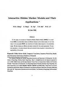
Empirical evidence suggests that the price process deviates from the semimartingale assumption in (1.1). The "volatility signature plot" (which shows (1.7) against sampling frequency, i.e., 1/n) in Figure (1.5) suggests a component in observed price that has an infinite quadratic variation. Previous authors have identified this component as microstructure noise, meaning that it is due to the fine grain structure of how observed prices are determined in financial markets. A common way of modelling this is as follows. Let Xtj be an observed log price and Ytj be discretely sampled from the process in (1.1). Then suppose that Xtj = Ytj + εtj ,

(1.8)

where εtj is a random error term. The simplest case is where the microstructure noise εtj is i.i.d with zero mean, independent of the process Y. This model was first considered in Zhou (1996) [105]. In this case, Zhang, Mykland, and Ait-Sahalia (2005) [104] showed that RV = 2nE(U 2 ) + Op (n1/2 ), which implies that RV is inconsistent and that divided by 2n it is an asymptotically unbiased estimator of the variance of microstructure noise. The noise can also be assumed to be serially correlated, and there are some theoretical results for this case, which we discuss below. One may want to allow for heteroscedasticity in (1.8), which has been taken up by Kalnina and Linton (2008) [76]. This is motivated by the stylized fact in market microstructure literature that intradaily spreads and intradaily stock price volatility are described typically by a U-shape (or reverse J-shape). See Andersen and Bollerslev (1997) [9], Gerety and Mulherin (1994), Harris (1986), Kleidon and Werner (1996), Lockwood and Linn (1990), and McInish and Wood (1992). Also to closely mimic the high frequency transaction data authors consider rounding error noise or non-additive noise that is generated from specific model of order book dynamics. Li and Mykland (2007) [81] discuss the rounding model; Xtj = log(δ[exp(Ytj + εtj )/δ]) ∨ log δ,

(1.9)

where δ[s/δ] denotes the value of s rounded to the nearest multiples of δ which is a small positive number. This is consistent with the market that has minimum price

ISSUES IN HANDLING INTRA-DAY TRANSACTION DATABASE

5

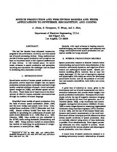
Time series plot of intraday price over a day

Figure 1.1

Time series plot of intra−day prices

High frequency Price

38.05

38

37.95 Trade Price Ask Bid

37.9

4000

6000

8000

10000

12000

14000

3900

4000

4100

4200

4300

4400

4500

change, tick sizes for stocks and futures markets and pip for foreign exchange market. The rounding model (1.9) is much more complex to work with than (1.8), due to the nonlinear way in which the efficient price enters. For example, even assuming no microstructure noise the quadratic variation of Xt is given by < f (Y ), f (Y ) >t where f (Y ) = E(X|Y ) is a complicated nonlinear function, although we are interested in estimating < Y, Y >t . Li et. al. (2007) [81] showed that when var(ε) is small, we have f (Yt ) ∼ Yt , whereas for a small noise variance, the divergence of two quadratic variations can be large. In any case, under the presence of such microstructure noise the Realized Variance is no longer a consistent estimator of the integrated variance. We explore the impact of different microstructure noise assumptions on RV and the class of consistent estimators under (1.1)-(1.8) in section 1.4.

1.3 ISSUES IN HANDLING INTRA-DAY TRANSACTION DATABASE Before examining volatility estimators based on high frequency data, it is important to understand the basic statistical features of such datasets. In this section we provide a brief summary of the stylized features of intra-day transaction data. The earlier papers of Goodhart and O’Hara (1997) [61] and Guillaume et. al. (1997) [66] provide early reviews. The distributional properties of high frequency returns varies with sampling frequency. At higher frequency, there is stronger evidence of a deviation from normality. Some common features, regardless of sampling schemes and the choice of trade and quote, are that the distribution of high frequency returns are approximately symmetric with large fourth moment. The empirical evidence suggests that the second moment is finite but the return distributions are fat-tailed with a distribution function whose tails decline according to a power law rather than a Gaussian distribution.

6


In fact, prices are discrete, meaning they are only quoted in integer multiples of tick size, which varies according to assets and time period (in the US tick size changed from being 1/8 of a dollar to 1/00th of a dollar during a few years at the beginning of the last decade), see Figure (1.1). However, returns, whether defined logarithmically or exactly, are less discrete, since the normalization changes over time, so this comment mostly just affects the study of prices within a single day. The returns of executed prices are negatively serially correlated. This is due to bid-ask bounce: at the tick level, buy orders are likely to be followed by sell orders and vice versa. Absolute returns and other activity variables such as volume, spread and trade duration exhibit short and long term memories. Andersen and Bollerslev (1997b) [8] showed that absolute trade returns, after eliminating the short term periodic component, has an autocorrelation function that has hyperbolic decay, i.e., have long memory. This can effect the construction of standard errors and forecasting. All of the variables associated with transaction activity show periodic patterns due to trading convention. The activity is high at the start and the end of the trading session and this induces a particular pattern in activity variables. Analyzing hourly data for multiple days reveals a strong hour of the day effect in activity variables. In addition, absolute returns have higher autocorrelation at the lags that are integer multiple of 5 minutes and periodically turns negative. The presence of periodicity has an important implication for modeling intra day series. For example, Andersen and Bollerslev (1997, 1997b) [9, 8] show that absolute returns show clear long memory only after adjusting for the periodic pattern. Periodicity can be modeled by introducing periodic dummies, frequency domain filtering and analysis at the activity time scale. The intra-day periodicity and long memory structure can be explained by the presence of an information arrival process that drives the price formation process. Hansen and Lunde (2005) [67] show how to treat the problem of intermittent data, such as in stock markets. They show the optimal way to combine the class of realized variance over the active trading portion of day and squared close to open returns. 1.3.1

Which price to use: Quote, Trade price, VWAP

Regarding intra-day data we typically have different types of prices: quote price, trade price and price reflecting order book information. Quotes are the prices that market participants are willing to buy (bid) and sell (ask). Quote returns are defined by a change in mid quotes, which is an average of bid and ask. Trade returns are the returns associated with the prices of executed trades. Note that in markets without a centralized exchange only the indicative quote data is available, indicative in the sense that it is non-binding. In terms of time series behavior, trade returns shows significant negative first order autocorrelation due to bid-ask bounce, since at the tick level buy orders are likely to be followed by sell orders and vice versa. In comparison, quote returns show positive first order autocorrelation in a short interval. See Figure (1.2). If the data is based on higher frequency sampling, for example at a tick time or one second, the quote and trade price have distinctively different features in returns and in absolute values. The difference disappears in lower frequency sampling. See Figure (1.3), which also shows that absolute returns are quite persistent. The VWAP


7

ACF of trade and quote return depending on sampling frequency

Figure 1.2

ACF: Highest Frequency

ACF: 10 minute

0.2

0.4

0.3

0.1

0.2 0

0.1 −0.1 0 −0.2 −0.1

−0.3 −0.2

trade return quote return −0.4

−0.5

−0.3

0

5

10

15

20

25

30

35

40

45

50

−0.4

0

2

4

6

8

10

12

14

16

18

20

(volume weighted average price), widely used by practitioners, is constructed as a weighted sum of quote price at different levels of order book where weight is given by the associated volume. Such price construction has the advantage that it uses more information available in the order book rather than just taking the first line of the order book, and discreteness is less severe than for the quote of trade price. This quantity is used in a common strategy for execution of large transactions, see Almgren and Chriss (2001) [7], and Engle, Ferstenberg, and Russell (2008) for example. One of the important conclusions we can draw from the analysis is that in ultrahigh frequency modelling, the choice of quote or trade price will sometimes affect the results of empirical modelling. For example, in calculating the naive realized variance measure of integrated variance based on low frequency returns, 10-20 minutes is a popular choice, in which case the choice of quote or trade returns will not have a discernible impact on the final quantity. However for more recently proposed methods that use all the data, we should compare the results using quote and trade returns. See Barndorff-Nielson et.al. (2008b) [24] for such studies.

1.3.2 High frequency data pre-processing Prior to analysis, the tick data has to be pre-processed to remove "non sensible" prices and duplicated transaction data points. Barndorff-Nielson et. al. (2008a) [24] provides a guideline for equity intra-day data. Brownlees and Gallo (2006) [39] summarize the structure of the TAQ high frequency data set and highlight some important aspects of the market procedures and address various issues in high frequency data management including: outlier detection and how to treat non-simultaneous observations, irregular spacing, issues of Bid Ask Bounce, and methods for identifying exact opening and closing prices. The authors also present the effect of data handling on

8


ACF of absolute trade and quote return depending on sampling frequency

Figure 1.3

ACF: Highest Frequency

ACF: 10 minute

0.3

0.4

absolute trade return absolute quote return

0.25

0.3

0.2 0.2

0.1 0.15 0 0.1 −0.1

0.05 −0.2

0

−0.05

−0.3

0

5

10

15

20

25

30

35

40

45

50

−0.4

0

2

4

6

8

10

12

14

16

18

20

fitting an ACD model to duration data. Bauwens and Giot (2001) provide a detailed description of the rules and procedures of the NYSE as well as other exchanges. For the market where there is a centralized exchange and trading is electronic the intra-day transaction data should be available easily. The example of such market is equities and commodity futures market. Where there is no centralized exchange, data providers provide the "indicative quote" stream. Most empirical work has so far concentrated on NYSE traded stocks and major currencies. Empirical application in other markets - geographically and also other fixed income markets will be of interest. 1.3.3

How to and how often to sample?

Intra-day prices are observed on the discrete and irregular intervals. For volatility estimation one can ask what is the effect of using all the data versus using sparsely sampled data, for example at 10-20 minutes. For covariance estimation, the problem is more substantial. Naturally the estimation of covariance involves the cross product of returns. How should we align the data points observed at a different times and what is the statistical impact of the synchronization method on the estimators? This section discuss two data sampling/alignment method: fixed clock time and refresh time method. We will present the synchronization method for d number of assets. The sampling method for univariate series is a special case for d = 1. In a given interval (for simplicity one day) [0, 1], we observe intra-day transaction prices of the i-th asset, Xi at discrete time points {ti,j ; j = 0, . . . , ni } where ni is a total number of observations on that interval. The set of {Xi,ti,j , ti,j ; i = 1, · · · , d, j = 1, . . . , ni }


9

gives us the tick database of prices for d numbers of assets. We can associate the counting process to {ti,j } Ni (t) :=

ni ∑

1(ti,j ≤ t)

j=1

recording the number of transactions that occurred for the i-th asset up to and including the time t. Let 0 = τ0 < · · · < τn = 1 be an artificially created time grid and let {si,j } be the actual time points of the data for i-th asset to be aligned on the {τj }’s grid. Regardless of how τ is defined we take the data that is closest to this artificial grid si,j = max {ti,l ≤ τj }. (1.10) 0≤l≤ni

We will denote an aligned dataset as {Xi,τj , τj ; i = 1, · · · , d, j = 1, · · · , n} with Xi,τj := Xi,si,j . If no observation is available during the given interval we repeat the previous data point. First, consider the problem of sampling scheme for univariate time series of intraday prices. One can use the raw tick data of prices observed at {ti,j } or work with instead sparser sampling. One method of sparse sampling is called fixed clock time. For example we might want to create one minute returns from the irregularly spaced tick data; τj = jh , h = 1/60 (1.11) so that τj −τj−1 = h, for all i. Empirical work shows that the effect of microstructure noise become attenuated when return are sparsely sampled. Ait-Sahalia, Mykland and Zhang (2005) [3] derived the optimal sampling rate h minimizing the mean square of the Realized Variance under the presence of i.i.d microstructure noise. When market microstructure noise is present but unaccounted for, they showed that the optimal sampling frequency is finite and derive its closed-form expression. The optimal sampling frequency is often found to be between one and five minutes. See Bandi and Russell (2008) [17] and reference therein for further discussion of optimal sampling rate in estimating integrated variance. However, modelling the noise and using all the data should yield a better solution, see section 104 on noise robust estimators. A second method for sparse sampling is to sample the price per given number of transactions. For example, data sampled per h number of transactions is τj+1 = ti,Ni (τj )+h

(1.12)

Griffin and Oomen (2008) [64] argued that under the transaction time sampling, returns are less serially correlated and microstructure noise is closer to i.i.d. They note the bias correction procedures that rely on the noise being independent are better implemented in transaction time. Figure (1.4) shows that the ACF of absolute returns at a different sampling scheme - verifying that the transaction time sampling scheme reduces the serial correlation and the process is closer to i.i.d.

10


Figure 1.4 ACF of absolute trade and quote return sampled by fixed clock time and transaction time ACF: absolute Trade Return

ACF: absolute Quote Return 0.25

0.12 Fixed Clock Time Alignment

0.1

Transaction Time Alignment

0.2

0.08

0.15

0.06

0.04 0.1 0.02 0.05 0

−0.02

0

−0.04 −0.05 −0.06

−0.08

0

5

10

15

20

25

30

35

40

45

50

−0.1

0

5

10

15

20

25

30

35

40

45

50

For the multivariate case, the additional issue of synchronicity arises, whereby trading for different assets occurs at different times. It is necessary to align the returns of asynchronously traded assets to calculate the covariance estimator that involves the cross product of returns. One method is to use the fixed clock time as given in (1.11). Another method, called the Refresh time, proposed by BarndorffNielsen, Hansen, Lunde and Shephard (2010) [25] can be thought as the multivariate version of the transaction time alignment given in (1.12). It is constructed by τj+1 = max {ti,Ni (τj )+1 } 1≤i≤d

(1.13)

As we sample the returns at higher frequency, zero returns (stale price) induce the downward bias in covariance estimators. This is known as the Epps effect. Hayashi and Yoshida (2005) [69] showed analytically a bias induced by the fixed clock time assuming independent homogenous Poisson process for Ni (t). The refresh time also induces synchronization bias and the problem is more severe for a high dimension covariance estimation since the method effectively collects the transaction time of the most illiquid asset. See Park et. al. (2010) [86] for further studies on the refresh time bias and its effect on the time domain based estimator of integrated covariance matrix. See the section (1.4.2) for a discussion of covariance estimator robust to the synchronization bias. 1.4 1.4.1

REALIZED VARIANCE AND COVARIANCE Univariate Volatility Estimators

We first present the results for realized volatility in the perfect world where there is no measurement error. The case of no noise is dealt with by Andersen, Bollerslev,

REALIZED VARIANCE AND COVARIANCE

Figure 1.5

11

Realized variance calculated at different calendar time frequencies

0.012

0.01

0.008

0.006

0.004

0.002

0

0

5

10

15

20

25

30

35

40

45

Sampling frequency

Diebold and Labys (2001) [11], Barndorff-Nielsen and Shephard (2002a, 2002b) [26, 27] and Mykland and Zhang (2006) [85]. Barndorff-Nielsen et al. (2002a) [26] showed that the error using the RV to estimate QV is asymptotically normal with rate √ n, i.e., ∫1 2 ∑ 2 √ j ytj − 0 σu du =⇒ N (0, 1), n √ ∫ 1 2 0 σu4 du where ytj = Ytj − Ytj−1 is the observed return and =⇒ is denote convergence in distribution. We remark that their proof does not require that Eyt4j < ∞ or even Eyt2j < ∞ as would generally be the case for a central limit theorem to hold. The reason is that the data generating process assumes a different type of structure, namely that locally the process is even Gaussian, and it is this feature that permits the arrival of the normal distribution in the limit. Note that this CLT is statistically infeasible since it involves a random unknown quantity called integrated quarticity ∫1 (IQ), 0 σu4 du. However we can consistently estimate this by the following sample quantity ∑ c =n IQ y 4 →p IQ. 3 j tj Therefore, the feasible CLT is given by √

This implies that ∫1 2 σ du. 0 u

∑ n

j

∫1 yt2j − 0 σu2 du √ =⇒ N (0, 1). c 2IQ

√ 2 c gives a valid α-level confidence interval for y ± z / 2IQ α/2 j tj

∑

12


1.4.1.1 Measurement Error Motivated by some of the issues observed in the intra-day financial time series largely to do with the presence of microstructure noise, authors have proposed competing estimators of the QV. The assumption on microstructure noise has been generalized from white noise to a noise process with one or many of following characteristics: autocorrelation, heteroskedacity, rounding models. McAleer and Medeiros (2008) [84] provide a summary of the theoretical properties of different estimators of QV under different assumptions of microstructure noise. Bandi and Russell (2006a) [19] have also reviewed the RV literature, with an emphasis on microstructure noise. Suppose that the efficient prices process is given by (1.1) and we observe (1.8). In this case, the realized variance is inconsistent. The first consistent estimators under this scheme was the two time scale estimator of Zhang, Mykland and Ait-Shahalia (2005) [104]. Let n−1 ∑( )2 [X, X]n = Xtj+1 − Xtj i=1

be the realized variation of observed log prices X. Split the sample of size n into K subsamples, with the ith subsample containing ni observations. Let [X, X]nj denote the j th subsample estimator based on a K-spaced subsample of size ni , and let [X, X]avg denote the averaged estimator: [X, X]ni =

n∑ i −1

(

XtjK+i − Xt(j−1)K+i

)2

, i = 1, . . . , K,

(1.14)

j=1

[X, X]avg =

K 1 ∑ [X, X]ni . K i=1

(1.15)

To simplify the notation, we assume that n is divisible by K and hence the number of data points is the same across subsamples, n1 = n2 = ... = nK = n/K. Let n = n/K. Define the adjusted TSRV estimator as ( ) n n = [X, X]avg − [X, X] . (1.16) n Zhang et. al. (2005) [104] show that this estimator is consistent and show that ( ) n1/6 < \ X, X >− < X, X > √ =⇒ N (0, 1) 8c−2 E 2 ε2 + cIQ provided that K = cn2/3 for any c ∈ (0, ∞). Zhang (2006) [102] extended this work to the multiscale estimator, which uses multiple time scale. She shows that this estimator is more efficient than the two time scale estimator and achieves the best convergence rate of Op (n1/4 ), (i.e., the same as the MLE with complete specification of the observed process).

REALIZED VARIANCE AND COVARIANCE

13

Kalnina and Linton (2008) [76] proposed a modification of the TSRV estimator that is consistent under heteroskedasticity and endogenous noise. A¨ıt-Sahalia, Mykland and Zhang (2010) [4] modified TSRV and MSRV estimators and achieve consistency in the presence of serially correlated microstructure noise. An alternative class of estimators is given by the so-called realized kernel estimators. The motivation for this class of estimators is to recognize the connection between the problem of estimating the long run variance of a discrete time process, Bartlett (1946) [29]. Define the symmetric realized autocovariance sequence γh (X) :=

n ∑

Xtj Xtj−h

(1.17)

j=h+1

for h = 0, ±1, . . . At zero lag γ0 (X) gives us the usual sum of squared high frequency returns, i.e., RV. The Kernel estimators smooth the realized autocovariance with weight function given by k(·), with k(0) = 1, k(s) → 0 as s → ∞ and the bandwidth H controls bias-variance trade-off. Specifically, consider ∑ ( h ) \ < X, X > = k γh (X). (1.18) H +1 |h|− < X, X > −c−2 |k ′′ (0)|E 2 ε2 √ =⇒ N (0, 1), (1.19) 4c||k||2 IQ ∫ provided that H = cn3/5 for any c ∈ (0, ∞), where ||k||2 := k(s)2 ds. The estimator is guaranteed to be positive definite. Note however, that the limiting distribution has a bias component. For inference, Zhang et. al. (2005) [104] n √ showed that [X,X] is n consistent estimator of Eε2 . The integrated quarticity 2n can be estimated by bipower type estimator of Barndorff-Nielsen and Shephard (2004) which is guaranteed to be positive definite but rate inefficient at Op (n1/5 ). In Barndorff-Nielsen et. al. (2008a) [23], they had a realized kernel estimator with a flat-top kernel i.e. k(0) = k(|1|/H) = 1 and the realized autocovariance γh was defined such that the sum runs from 1 not h + 1. Their flat top realized kernel was

14


unbiased under the presence of i.i.d microstructure noise and achieves the optimal convergence rate, Op (n1/4 ). The drawback of the earlier version, however is that the resulting estimator is not guaranteed to be p.s.d. We should briefly mention the promising pre-averaging method analyzed for example in Jacod, Li, Mykland, Podolskij and Vetter (2009) [73], which involves averaging observed prices over a moderate number of time points to reduce the measurement error. Consider Xt =

1 nt

∑

Xtj

|t−tj | = [Y , Y ] − [Y1 , Y2 ] . 1 2 1 2 nJ with the average lag K realized covariance is defined by [Y1 , Y2 ]K =

n 1 ∑ (Y1,τj − Y1,τj−K )(Y2,τj − Y2,τj−K ) K j=K

This is consistent and Op (n1/6 ) asymptotically normal under the presence of noise and asynchronous trading.

18


Barndorff-Nielsen et al. (2010) [25] proposed to synchronize the high frequency prices using Refresh Time explained in section 1.3.3. They assumed that the microstructure noise {ϵi,τj , i = 1, . . . , d} is a second order stationary with respect to refresh time {τj }. Their Multivariate Realized Kernels (MRK) is given in (1.18) with realized autocovariance defined by ∑ γh (X) = xτj xTτj , j

where x = [x1 : · · · xd ] is a matrix of refresh time aligned returns for d number of assets. The MRK is Op (n1/5 )−consistent and asymptotically normal and its asymptotic distribution is given in (1.19) under second order kernel. It is also guaranteed to be positive semi definite Ait Sahalia, Fan and Xiu (2010) [1] proposed O(n1/4 ) consistent estimator based on the QMLE and a generalized time synchronization method. An advantage of their estimator over TSCV and MRK that it does not involve estimating tuning parameters such as bandwidth. However they adopt somewhat restrictive assumption on the microstructure noise - white noise which is mutually independent across assets. Christensen, Kinnebrock and Podolskij (2010) [46] proposed a multivariate preaveraging estimator. Voev and Lunde (2007) [98] proposed a modified Hayashi and Yoshida estimator to bias-correct for the microstructure noise, but the estimator does not achieve consistency. See Bauer and Borkink (2008) [30] for latent factor model of realized covariance matrix. Park and Linton (2010) [86] proposed a covariation estimator that is microstructure noise and synchronization robust based on fourier analysis of returns, extending Mallianvin and Mancino (2009) [83]. Griffin and Oomen (2011) [65] ranks the performance in terms of efficiency of the three estimators; realized covariance, realized covariance plus lead- and lag-adjustments, and the Hayashi and Yoshida estimator. They found that performance of competing estimators depends on the level of microstructure noise as well as the level of correlation. 1.5

MODELLING AND FORECASTING

In this section, we review methods for modelling the time series of Realized Volatilities and summarize the studies that compare these models in terms of forecasting power where the forecasting variable is a general function of volatility such as VaR or portfolio performance. Also we consider extensions to a dynamic model of the realized covariance matrix. See other chapters of this handbook on more detailed survey on this area. 1.5.1

Time series models of (co) volatility

Once we have an estimator of the integrated variance we can consider time series modeling and forecasting it. The unobserved component model is considered by

MODELLING AND FORECASTING

19

Barndorff-Nielsen and Shephard (2002) [26] and Koopman, Jungbacker, and Hol (2005). The key feature of the time series of RV is that it is highly persistent. To account for this, Andersen, Bollerslev, Diebold, and Labys (2003) [12] use autoregressive fractionally integrated model(ARFIMA). Let ht denote an estimator of integrated variance for t-th day. Θ(L)(1 − L)d (ht − µ) = ϵt ∼ WN(0, 1),

(1.23)

where Θ(L) is a polynomial of lag operators and d is a degree of fractional integration. The modified ARFIMA with time varying parameters and a non-Gaussian error is put forward by Lanne (2006) [80]. The temporal dependence in the estimator of variance can be modelled parsimoniously by the Heterogenous Autogressive model of Coris (2009) [50], which is given by (W )

ht+1 = β0 + βD ht + βW ht

(M )

+ βM h t

+ ϵt+1 ,

(W )

where ht := 15 (ht + · · · + ht−4 ) is a realized variance over a week and similarly (M ) defined ht denotes the realized variance over a month. Liu and Maheu (2009) [82] consider Bayesian averaging over both different measures of integrated variance and different time series models. See also the HEAVY model of Shephard and Sheppard (2010) [94] and the Mixed data sampling by Ghysels et. al. (2006) [59]. For time series modelling the integrated covariance matrix, Voev (2007) combined the univariate variance and covariance forecasts to produce a positive definite matrix forecast. Gourieroux, Jasiak, and Sufana (2009) [63] proposed the Wishart Autoregressive (WAR) model for covariance matrix which accommodates the positivity and symmetry of volatility matrices. Bauer and Vorkink (2011) [31] employed the matrix log transformation to guarantee positive definiteness of the forecast. For time series model for such transformed data, they adopted a latent factor model where forecasting variables are lagged covariances, lagged returns and other forecasting variables. Chiriac and Voev (2010) [44] carried out a Cholesky decomposition of covariance matrix and model the lower dimensional factor covariance matrix by a multivariate vector fractionally integrated ARMA (VARFIMA). They showed their method outperforms using HAR model, Dyanamic Conditional correlation model and its fractionally integrated counterpart using limited number of stocks. 1.5.2 Forecast comparison Since volatility itself is unobservable, the comparison of volatility forecasts rely on an observable proxy for latent volatility process. See Patton (2011) [88] on a method that is robust to the presence of measurement error in the volatility proxy. Authors have conducted forecast comparisons of time series models of RV with different forecasting objects. Brownlees and Gallo (2009) [40] compared the Value at Risk forecasts from different time series models of RV. Bandi, Russel and Yang (2008a) [20] considered the comparison in the context of option pricing, while Voev (2009) did this in the context of unconditional measure of portfolio performance.

20


We are also interested in comparing the dynamic model of estimators of ex-post variation calculated from the high frequency data on the one hand, and an entirely different class of volatility estimators - e.g., the class of GARCH and implied volatility on the other. Koopman, Jungbacker and Hol (2005) [78] compared the historical volatility from a daily return series, the implied volatility from options and the realized volatility, combined with the functional forms of unobserved component, long memory, stochastic volatility and GARCH. The long memory model with realized volatility seems to have the most forecasting power. Hansen and Lunde (2005) [67] and Shephard and Sheppard (2010) [94] compared the dynamic models of RV to GARCH. A comparison is made to EGARCH by Maheu and McCurdy (2009). Siu and Okunev (2009) compared historical, realized and implied volatility measures for predicting over multiple horizons. The role of microstructure noise on forecasting performance is discussed by Ait-Shahlia and Mancini (2006) [2] and Ghysels and Sinko (2011) [60]. In Dimitrios (2003), the authors presents the forecast comparison using the high frequency data from the futures on stocks, bond and foreign exchange markets. 1.6 1.6.1

ASSET PRICING Distribution of returns conditional on the volatility measure

There is a literature that documents evidence that the de-volatized returns by the class of RV estimators are Gaussian or approximately so. Andersen, Bollerslev, Diebold and Labys (2001) [11] found that daily returns standardized by the realized volatility approximate the Gaussian distribution. Thomakos and Wang (2003) [96] also found such evidence for a futures market. Peters and de Vilder (2006) [89] studied the volatility and return dependence by sampling the returns in financial time. They tested if the return series are a realization of a local martingale using the theorem by Dubins and Schwarz (1965) [53] who stated that any continuous local martingale Xt ∈ Ft is a time-changed Brownian motion. Formally stated, Bs = XTs , Ts = inf{t|[X]t ≥ s}, (1.24) where Bs ∈ FTs is a Brownian motion. Ts is a stopping time constructed by recording the first time the quadratic variation reaches a specified level. Equivalently the theorem implies that X can be represented as Xt = B[X]t .

(1.25)

The equation (1.25) states that every continuous martingale is a time changed Brownian motion where the time change is given by the quadratic variation. In empirical analysis, (1.24) is more relevant, which states that between the unit interval of the transformed time, [T ((i − 1)a), T (ia)], X has a constant QV at a. Given an interval of physical time, X is sampled more frequently when QV is large. More precisely, the transformed time, Tt is constructed by, T0 = 0, Tj = Tj−1 + ∆Tj , and ∆Tj = inf{t|[X](Tj−1 ,Tj−1 +t) ≥ a},

(1.26)

ASSET PRICING

21

where [X](Tj−1 ,Tj−1 +t) denotes the quadratic variation between [(Tj−1 , Tj−1 + t)). The standardized increment in financial time ξ=

X(Tj ) − X(Tj−1 ) √ a

(1.27)

is i.i.d standard normal. Observe the trade-off between having large and small a. We need to have large a to have many data points to consistently estimate QV by Realized Variance but large a means sparse sampling of X. Note also that we can explicitly derive the distributional features of the stopping time T when the X process is completely specified. Testing for the hypothesis that Xt is a local martingale is then equivalent to a testing for i.i.d standard normality of the return series that is spaced by Ts . Peters and de Vilders (2006) [89] tested if the S & P 500 intra-day return is a local martingale where they constructed the stopping time Ts based on the Realized Variance. They concluded that we cannot reject the null hypothesis that returns are the realization of a martingale process at various time scales (> 1 day) based on the tests for Gaussianity, independence and serial correlation. A similar study was done by Jeong and Park (2008) who constructed stopping times using the jump robust QV estimator such as the bi-power variation. Andersen et al (2007) extended their approach for the presence of jumps. Similar issues studied in Fleming et. al. (2006) and Mahew and McCurdy (2002). 1.6.2 Application to factor pricing model The K factor pricing model for stock returns yi is given by yit = βi⊤ ft + εtt ,

(1.28)

where the factor loadings βi = (βi1 , . . . , βiK )⊤ are unrestricted, Ross (1976) [93]. Here, the sampling unit is typically low frequency and cross-sectional with i = 1, . . . , n indexing firms and t = 1, . . . , T indicating low frequency time scale like monthly. In some cases ft are unobserved statistical factors, while in others they are the returns on observed carefully constructed portfolios, Fama and French (1993) [54]. In this latter case, βj,k can be given the interpretation of the covariance between return on portfolio j and asset i divided by the variance of the return on asset j. There is a lot of recent work in which the betas are allowed to be time varying according to certain specifications. The continuous time framework allows us to measure the realized beta between two assets in a certain time period using high frequency data. In general, the beta between asset k and l using high frequency returns can be estimated by the realized beta in period [t − 1, t] from high frequency data ∫t ∑ Σ(k,l) (s)ds xk,j xl,j j βˆk,l (t) = ∑ 2 →p ∫t−1 ≡ βk,l (t), t Σ (s)ds j xl,j (l,l) t−1 where the convergence in probability holds under the absence of noise as the number of high frequency observations in the period [t − 1, t] goes to infinity. For studies

22


on the relationship between return and volatility, see Ghosh and Linton (2007) [62], Bollerslev, Litvinova, and Tauchen (2006) [33] and Bali and Peng (2006) [16]. Ghosh and Linton (2007) [62] showed that the estimation problem for the risk-return trade-off parameters can be posed as a GMM estimation problem. They used the RV as a conditional volatility proxy. Their empirical results suggested significant time-variation in the risk-return slope coefficient. Bali et. al. (2006) [16] found a positive and statistically significant relation between the conditional mean and conditional volatility of market returns at the daily level where volatility is proxied by RV. Bollerslev et. al. (2006) [33] made use of the time aggregation formula between lower and high frequency covariance. They found that the correlations between absolute high-frequency returns and current and past high-frequency returns are significantly negative for several days. Andersen, Bollerslev, Diebold and Wu (2005) [13] and Bandi and Russell (2005) estimated the beta in CAPM by a realized covariation. Bandi et.al. (2005) [18] provide a MSE-based optimal sampling frequency method for calculating the realized beta designed to reduce the effect of market microstructure noise. Bollerslev and Zhang (2003) [34]estimated factor loadings in the three-factor Fama-French model by high frequency based estimator with a simple adjustment procedure to account for nonsynchronous trading effects. Bannouh, Martens, Oomen and van Dijk (2009) [21] and Kyj , Ostdiek and Ensor (2009) [79] used mixed frequency framework ; using the high-frequency data to obtain an estimate of the factor covariance matrix and using the daily data to estimate the factor loadings. This method avoids the non-synchronicity problems inherent in the use of high frequency data for individual stocks. The economic value of using the realized covariance in portfolio management is discussed by Fleming et.al. (2003) [56], De Pooter et.al. (2008), Liu (2009) and Bandi et.al. (2007) [22]. Fleming et.al. (2003) and De Pooter et.al. (2008) find that a risk-averse investor is willing to pay between 50 and 200 basis points per annum to switch to a covariance measurement based on daily data to intraday data. Pooter et.al. (2008) investigate the benefits of high frequency intraday data when constructing the mean-variance efficient portfolio. Liu (2009) examine how the use of high-frequency data impacts the portfolio optimization decision. Bandi et.al. (2007) discuss volatility-timing trading strategies relying on optimally-sampled realized variances and covariances. They consider stock portfolios with daily re-balancing from the individual constituents of the S&P100 index. They focus on the issue of determining the optimal sampling frequency as judged by the performance of these portfolios. Fan, Li and Yu (2010) [55] studied the volatility matrix estimation using high-dimensional high-frequency data from the perspective of portfolio selection. Specifically, they proposed the use of "pairwise-refresh time" and "all-refresh time" for estimation of vast covariance matrix and compared their merits in the portfolio selection and showed that advantage of using high-frequency data is significant in their simulation and empirical studies.

ASSET PRICING

23

1.6.3 Effects of Algorithmic Trading Recently, the effects of high frequency or algorithmic trading have been the focus of policy discussions, arising part from the recent flash crash of May 2010, where the US market suffered massive and rapid price decreases followed ultimately by a recovery. Chaboud et al. (2009) [43] investigate the effects of algorithmic trading on volatility. They consider high frequency exchange rate data from the EBS system for currency i = 1, 2, 3. They consider the following regression equation RVit = αi + βi ATit + γi⊤ τit +

22 ∑

δik RVi,t−k + εit ,

k=1

where RVit is the log of realized volatility of currency i during day t computed using one minute returns, ATit is the fraction of trading that was implemented using computers in that day and currency, which was recorded by the trade matching engine, and τit are dummy and time trend variables. The latter are included because the AT series has a pronounced upward trend, while volatility appears more or less stationary. They recognized the endogeneity issue that high frequency automated trading algorithms may trade more in volatile times so that AT is endogenous; they therefore instrument it with an instrument that measures the capacity for computer trading in a given currency/period combination, measured at the quarterly frequency. They find that the estimation strategy matters here, so that using OLS yields a positive effect, βi > 0, but the instrumental variable estimator finds βi < 0 but not statistically significant. The conclude that intraday algorithmic trading does not by itself lead to higher daily volatility. Some other studies that use some measure of volatility to determine the effects of HFT are: Hendershott, Jones and Menkveld (2009) [70], Hendershott and Riordan [71] (2009), and Brogaard (2010) [38]. Finally, we should mention related work of Ait-Sahalia and Yu (2009) [5] who investigate the relationship between the noise component of RV and liquidity measures. 1.6.4 Application to Option pricing In recent years, volatility is started to be thought as asset class on its own and an investment instrument has been developed. One can trade volatility through position in puts and calls but this has additional exposure to price movement. Swaps and options on quadratic variation have been developed for pure exposure on the volatility. For a discussion of volatility as an asset class, see Demeterfi, Derman, Kamal, and Zou (1999) [51]. Volatility swap is a forward contract on annualized volatility. Its payoff at expiration is equal to (RVt,T − SWt,T )N. The floating leg RVt,T is usually is a sum of squared daily log returns, which differs from the quadratic variation of the log price by the sampling frequency. Note the difference in terminology - we so far referred RV as sum of squared high frequency returns, but here sampling frequency is lower. N is the notional amount of the swap

24


in dollars per annualized volatility point. Investor for such instrument is swapping a fixed volatility SWt,T for the actual (\floating") future volatility RVt,T . The value of a forward contract F on quadratic variation, [Y ]t,T (denoting QV accumulated over [t, T ]) with strike SWt,T with r denoting a risk-free discount rate corresponding to the expiration T is the expected present value of the future payoff: F = E Q [erT ([Y ]t,T − SWt,T )]. Then the strike for which the contract has zero present value is; ∗ SWt,T = E Q ([Y ]T ).

Carr et. al. (2005) [41] proposed a method of pricing options on quadratic variation via the Laplace transform when returns are assumed to follow pure jump Levy processes. Itkin and Carr(2010) [72] considered return process that follows time changed levy process. Britten-Jones and Neuberger(2000) [37] proposed a method to estimate the optionimplied (i.e., risk-neutral) integrated variance over the life of the option contract; E Q ([Y ]T ) when prices are continuous with stochastic volatility and Jiang and Tian ∗ (2005) [75] showed the accuracy of the method when prices has jumps. SWt,T is considered \model-free,’ and can be labeled the model-free implied variance (MFIV) as well as being a no-arbitrage variance swap rate. Carr and Wu [42] show that the variance swap rate, is well approximated by the value of a particular portfolio of options. They established that the difference between the realized variance and this synthetic variance swap rate ∗ RVt,T − SWt,T to quantify the variance risk premium. They have analysed the variance swaps for stocks and found to be significantly negative . This means that investors are willing to pay a premium to hedge away upward movement in the return variance. Bollerslev et al. [32] proposes a method for constructing a volatility risk premium relying on the sample moments of the realized variance and option-implied volatility measures. Wu (2010) [100] studied the variance dynamics and variance risk premium using both the variance swap rate constructed from the options and the quadratic variance estimates using the high frequency data and found a strong evidence for negative VRP in equity markets. For bond markets, Wright and Zhou [99] found that the incremental return predictability captured by the realized jump mean largely accounts for the countercyclical movements in bond risk premia. For the research studying the pricing of volatility risk in individual stock options ; Driessen et al. (2009) [52] found that cross-sectional differences in exposure to market wide correlation risk can account for differences in expected option returns. Bakshi and Kapadia [15] found evidence of negative risk premium by examining the delta hedged option portfolio. For how class of QV estimators are used in pricing options on cash instrument, see Stentoft (2008) [95] ,Christoffersen et. al. (07,2010) [48], [47]. For correlation swap valuation see Jacquier (2007) [74].

25

APPLICATION TO ESTIMATING CONTINUOUS TIME MODELS

1.7 APPLICATION TO ESTIMATING CONTINUOUS TIME MODELS In this section we review how class of QV estimators are used to estimate the parameters in continuous time models. Consider a model for financial prices Xt dXt = µ(Xt , θ)dt + σ(Xt , θ)dBt

(1.29)

where B is independent Brownian motion. We are interested in estimating θ. The example of such process is geometric Brownian motion, OU process and CIR process. Xt is non-homogenous in a sense that diffusion coefficient is non constant and function of Xt . Since Xt is Markov we can write down a log likelihood in terms of transition density if closed form exists. When Xt is observed continuously, the likelihood function for the continuous record can be obtained via Girsanov theorem; see Phillip and Yu (2009) [90] on survey of literature for estimating model (1.29) using maximum likelihood. However in practice we observe the data at discrete time points and even for densely sampled high frequency data, it deviates from the model in (1.29) due to a presence of microstructure noise. Phillip and Yu (2009) [91] proposed a two stage estimation method for (1.29) based on discretely observed data; In the first stage, they estimate the diffusion coefficient using the microstructure noise robust estimator of integrated variance. Next the parameters of the drift component are estimated by the infill likelihood. Their estimator is rate efficient under infill and mixture of infill and long span asymptotics. The time changed Brownian motion given in (1.24) can be also used to construct an exact Gaussian maximum likelihood for a non-homogeneous ito-process as shown by Yu and Philips (2001) [101]. Once the model departs from Markov property in (1.29), for example in stochastic volatility models, we cannot decompose the likelihood into transition density. Bollerslev and Zhou (2002) [35] proposed a GMM type estimator for the underlying model parameters of stochastic volatility model by matching the sample moments of the realized volatility to the population moments of the integrated volatility implied by a particular continuous-time model structure. Corradi and Distaso (2006)[49] provide theoretical justification for such a GMM estimator. Barndorff-Nielsen and Shephard (2002a) [26] used the quasi-likelihood in the case where the model can be handled by the Kalman filter. Barndorff-Nielsen and Shephard (2006b) [28] used QML to estimate the parameters (related to moments) of the continuous time model using RV, assuming normality of quadratic variation. Todorov [97] proposes a method of inference for general stochastic volatility models containing price jumps. The estimation is based on treating realized multipower variation statistics calculated from high-frequency data as their unobservable in-fill asymptotic limits.

REFERENCES 1. Y. Ait-Sahalia, J. Fan, and D. Xiu. High frequency covariance estimates with noisy and asynchronous financial data. Journal of American Statistical Association, 94:9–51, 2010.

26


2. Y. Ait-Sahalia and L. Mancini. Out of sample forecasts of quadratic variation. Working Paper, Princeton University and University of Zurich, 2006. 3. Y. Ait-Sahalia, P.A. Mykland, and L. Zhang. How often to sample a continuous-time process in the presence of marketmicrostructure noise. Review of Financial Studies, 18:351–416, 2005. 4. Y. Ait-Sahalia, P.A. Mykland, and L. Zhang. Ultra high frequency volatility estimation with dependent microstructure noise. Journal of Econometrics, 2010. forthcoming. 5. Y. Ait-Sahalia and J. Yu. High frequency market microstructure noise estimates and liquidity measures. Annals of Applied Statistics, 3(1):422–457, 2009. 6. S. Alizadeh, M.W. Brandt, and F.X. Diebold. Range-based estimation of stochastic volatility models. Journal of Finance, 57:1047–1091, 2002. 7. Almgren and Chriss. Optimal execution of portfolio transactions. 2001. 8. T.G. Andersen and T. Bollerslev. Heterogeneousinformation arrivals and return volatility dynamics: uncovering the long-run in high frequency returns. Journal of Finance, 52:975–1005, 1997. 9. T.G. Andersen and T. Bollerslev. Intraday periodicity and volatility persistence in financial markets. Journal of Empirical Finance, 4:115–158, 1997. 10. T.G. Andersen, T. Bollerslev, F.X. Diebold, and P. Labys. Exchange rate returns standardized by realized volatility are (nearly) gaussian. Multinational Finance Journal, 4:159–179, 2000. 11. T.G. Andersen, T. Bollerslev, F.X. Diebold, and P. Labys. The distribution of exchange rate volatility. Journal of the American Statistical Association, 96:42–55, 2001. 12. T.G. Andersen, T. Bollerslev, F.X. Diebold, and P. Labys. Modeling and forecasting realized volatility. Econometrica, 71:579–625, 2003. 13. T.G. Andersen, T. Bollerslev, Diebold F.X., and G. Wu. Aframework for exploring the macroeconomic determinants of systematic risk. American Economic Review, 95:398– 404, 2005. 14. K. Back. Asset pricing for general processes. Journal of Mathematical Economics, 20:371395, 1991. 15. G. Bakshi and N. Kapadia. Delta-hedged gains and the negative market volatility risk premium. Review of Financial Studies, 16:527–566, 2003. 16. T.G. Bali and L. Peng. Is there a risk-return tradeoff? Working paper, Zicklin School of Business, 2006. 17. F. M. Bandi and B. Perron. Long-run risk-return trade-offs. Journal of Econometrics, 143(2):349–74, 2008c. 18. F. M. Bandi and Russell J. R. Realized covariation, realized beta and microstructure noise. Working Paper, Graduate School of Business, University of Chicago, 2005. 19. F. M. Bandi and Russell J. R. Market microstructure noise, integrated variance estimators, and the limitationsof asymptotic approximations: A solution. Working Paper, Graduate School of Business, University of Chicago, 2006a. 20. F. M. Bandi, J. R. Russell, and C. Yang. Realized volatility forecasting and option pricing. Journal of Econometrics, 147(1):34–46, 2008a.

REFERENCES

27

21. K. Bannouh, M. Martens, R. Oomen, and van Dijk D. Realized factor models for vast dimensional covariance estimation. Working paper, University Rotterdam, 2009. 22. R. Bansal and A. Yaron. Risks for the long run: a potential resolution of asset pricing puzzles. Journal of Finance, 59:1481–1509, 2004. 23. O. Barndorff-Nielsen, P.R. Hansen, A. Lunde, and Shephard N. Designing realized kernels to measure the ex-post variation ofequity prices in the presence of noise. Econometrica, 76:1481–536, 2008. 24. O. Barndorff-Nielsen, P.R. Hansen, A. Lunde, and Shephard N. Realized kernels in practice: trades and quotes. Econometrics Journal, 4:1–32, 2008. 25. O. Barndorff-Nielsen, P.R. Hansen, A. Lunde, and Shephard N. Multivariate realised kernels: consistent positive semi-definiteestimators of the covariation of equity prices with noise and non-synchronous trading. Journal of Econometrics, 2010. forthcoming. 26. O. Barndorff-Nielsen and N. Shephard. Econometric analysis of realised volatility and its use in estimating stochastic volatility models. Journal of the Royal Statistical Society, Series B, 64:253–280, 2002a. 27. O. Barndorff-Nielsen and N. Shephard. Econometric analysis of realised covariation:high frequency covariance, regression and correlation in financialeconomics. Econometrica, 72:885–925, 2002b. 28. O. Barndorff-Nielsen and N. Shephard. Impact of jumps on returns and realised variances: econometric analysis of time-deformed lévy processes. Journal of Econometrics, 131:217–252, 2006b. 29. M. S. Bartlett. On the theoretical specification of sampling properties of autocorrelated time series. Journal of the Royal Statistical Society, Supplement, 8:274, 1946. 30. G. H. Bauer and K. Vorkink. Multivariate realized stock market volatility. Bank of Canada and Brigham Young University, 2008. 31. G. H. Bauer and K. Vorkink. Forecasting multivariate realized stock market volatility. Journal of Econometrics, 160:93101, 2011. 32. T. Bollerslev, M. Gibson, and H. Zhou. Dynamic estimation of volatility risk premia and investor risk aversion fromoption-implied and realized volatilities. Journal of Econometrics, 2010. forthcoming. 33. T. Bollerslev, J. Litvinova, and G. Tauchen. Leverage and volatility feedback effects in high-frequency data. Journal of Financial Econometrics, No. 3, 4:353384, 2006. 34. T. Bollerslev and Y. B Zhang. Measuring and modeling systematic risk in factor pricing models using high-frequency data. Journal of Empirical Finance, 10(5):533–558, 2003. 35. T. Bollerslev and H. Zhou. Estimating stochastic volatility diffusion using conditional moments of integrated volatility. Journal of Econometrics, 109:33–65, 2002. 36. M. W. Brandt and F. X. Diebold. A no-arbitrage approach to range-based estimation of return covariances and correlations. Journal of Busines, 79:61–73, 2006. 37. M. Britten-Jones and A. Neuberger. Option prices, implied price processes, and stochastic volatility. Journal of Finance, 55:839–866, 2000. 38. J.A. Brogaard. High frequency trading and its impact on market quality. PhD thesis, Northwestern University, October 2010.

28


39. C. T. Brownlees and G. M. Gallo. Financial econometric analysis at ultra-high frequency: Data handling concerns. Working Paper, 2006. 40. C. T. Brownlees and G. M. Gallo. Comparison of volatility measures: a risk management perspective. Journal of Financial Econometrics, pages 1–28, 2009. 41. P. Carr, H. Geman, D. B. Madan, and M. Yor. Pricing options on realized variance. Finance and Stochastics, 9:453475, 2005. 42. P. Carr and L. Wu. Variance risk premia. Review of Financial Studies, 22(3):1311–1341, 2009. 43. A. Chaboud, B. Chiquoine, E. Hjalmarsson, and C. Vega. Rise of the machines: Algorithmic trading in the foreing exchange market. Board of Governors Internation Finance Discussion paper no 980., 2009. 44. R. Chiriac and V Voev. Journal of Applied Econometrics. Forthcoming. 45. K. Christensen and M. Podolskij. Realised range-based estimation of integrated variance. Journal of Econometrics, 141:323–349, 2007. 46. K. Christensen, Kinnebrock S., and M. Podolskij. Pre-averaging estimators of the expost covariance matrix in noisy diffusion models with non-synchronous data. Journal of Econometrics, 159:116–133, 2010. 47. P. Christoffersen, R. Elkamhi, B. Feunou, and K. Jacobs. Option valuation with conditional heteroskedasticity and nonnormality. Review Financial Studies, 23(5):2139–2183, 2010. 48. P. F. Christoffersen, K. Jacobs, and K. Mimouni. Models for s&p 500 dynamics: evidence from realized volatility, daily returns, andoption prices. Working Paper, Mcgill University, 2007. 49. V. Corradi and W. Distaso. Semi-parametric comparison of stochastic volatility models using realized measures. Review of Economic Studies, 73:635–667, 2006. 50. F. Corsi. A simple long memory model of realized volatility. Journal of financial econometrics, 7:174–196. 51. K. Demeterfi, E. Derman, M. Kamal, and J Zou. More than you ever wanted to know about volatility swaps. Technical report, 1999. Research notes, Goldman Sachs. 52. J. Driessen, P. Maenhout, and G. Vilkov. Option-implied correlations and the price of correlation risk. Journal of Finance, 64(3):1377–1406, 2009. 53. L. Dubins and G. Schwartz. On continuous martingale. Proceedings of the National Academy of Sciences of the United States of America, 1965. 54. E.F. Fama and K.R. French. Common risk factors in the returns to stocks and bonds. Journal of financial economics, 33:3–56, 1993. 55. J. Fan, Y. Li, and K. Yu. Vast volatility matrix estimation using high frequency data for portfolio selection. Working Paper, 2010. 56. J. Fleming, C. Kirby, and B. Ostdiek. The economic value of volatility timing using realized volatility. Journal of Financial Economics, 67:473–509, 2003. 57. L. Forsberg and E. Ghysels. Why do absolute returns predict volatility so well? Journal of Financial Econometrics, 5:31–67, 2007. 58. J. Gatheral and Oomen R.C.A. Zero-intelligence realized variance estimation. Finance and Stochastics, 14:249283, 2010.

REFERENCES

29

59. E. Ghysels, P. Santa-Clara, and R. Valkanov. Predicting volatility: how to get the most out of returns data sampled at different frequencies. Journal of Econometrics, 131:59–95, 2006. 60. E. Ghysels and A. Sinko. Volatility forecasting and microstructure noise. Journal of Econometrics, 160:257271, 2011. 61. C. Goodhart and M. O’Hara. High frequency data in financial markets: Issues and applications. Journal of Empirical Finance, 4:73–114, 1997. 62. A. Gosh and O. Linton. Consistent estimation of the risk-return tradeo⁄in the presence of measurement error. Working paper, London School of Economics, 2007. 63. C. Gourieroux, J. Jasiak, and R. Sufana. The wishart autoregressive process of multivariate stochastic volatility. Journal of Econometrics, 150:167–181, 2009. 64. J.E. Griffin and R. C. A. Oomen. Sampling returns for realized variance calculations: tick time or transaction time? Econometric Reviews, 27(1-3):230–253, 2008. 65. J.E. Griffin and R. C. A. Oomen. Covariance measurement in the presence of non- synchronous trading and market microstructure noise. Journal of Econometrics, 160:5868, 2011. 66. D. M. Guillaume, M. M. Dacorogna, R. R. Dave, U.A. Muller, and R. B. andPictet O. V. Olsen. From the bird’s eye to the microscope: A survey of new stylized facts of the intra-daily foreign exchange markets. Finance Stochastitcs, 1:95–129, 1997. 67. P. R. Hansen and A. Lunde. A realized variance for the whole day based on intermittent high-frequency data. Journal of Financial Econometrics, 3:525–554, 2005. 68. P. R. Hansen and A. Lunde. Realized variance and market microstructure noise. Journal of Business & Economic Statistics, 24:127–161, 2006. 69. T. Hayashi and N. Yoshidam. On covariance estimation of non-synchronously observed diffusion processes. Bernoulli, 11:359–379, 2005. 70. T. Hendershott, C. Jones, and Menkveld A. Does algorithmic trading improve liquidity? Working Paper, 2010. 71. T. Hendershott and R. Riordan. Algorithmic trading and information. NET Institute, working paper #09-08, 2009. 72. A. Itkin and P. Carr. Pricing swaps and options on quadratic variation under stochastic time change modelsdiscrete observations case. Review of Derivative Research, 13:141176, 2010. 73. J. Jacod, Y. Li, P. A. Mykland, Podolskij M., and Vetter M. Microstructure noise in the continuous case: the pre-averaging approach. Stochastic Processes and Their Applications, 119:2249–2276, 2009. 74. Jacquier. Variance dispersion and correlation swaps. Jacquier, A. and Slaoui, S., 2007. 75. G. J. Jiang and Y. S. Tian. The model-free implied volatility and its information content. Review of Financial Studies, 18(4):130542, 2005. 76. I. Kalnina and O. Linton. Estimating quadratic variation consistently in the presence of correlated measurement error. Journal of Econometrics, 147:47–59, 2008. 77. I. Karatzas and S. Shreve. Brownian Motion and Stochastic Calculus. 1991. 78. S.J. Koopman, B Jungbacker, and E. Hol. Forecasting daily variability of the s&p 100 stock index using historical, realised and implied volatility measurements. Journal of Applied Econometrics, 20(2):311–323, 2005.

30


79. L. Kyj, B. Ostdiek, and K. Ensor. Covariance estimation in dynamic portfolio optimization: A realized single factor model. Working Paper, 2009. 80. M. Lanne. A mixture multiplicative error model for realized volatility. Journal of Financial Econometrics, 4(4):594616, 2006. 81. Y. Li and P. A. Mykland. Are volatility estimators robust with respect to modeling assumptions? Bernoulli, 13(3):601–622, 2007. 82. C. Liu and J. M. Maheu. Forecasting realized volatility: a bayesian model-averaging approach. Journal of Applied Econometrics, 24:709–733, 2009. 83. P. Malliavin and M. E. Mancino. Fourier series method for nonparametric estimation of multivariate volatility. The Annals of Statistics, 37(46):1983–2010, 2009. 84. M. McAleera and M. C. Medeirosb. Realized volatility. A Review Econometric Reviews, 27(1-3):10–45, 2008. 85. P. A. Mykland and L. Zhang. Anova for diffusions and ito processes. The Annals of Statistics, 34(4):1931–1963, 2006. 86. S. Park and O. Linton. A fourier domain approach to integrated (co)volatility estimation. 2010. Working Paper. 87. M. Parkinson. Journal of business. The extreme value method for estimating the variance of the rate of return, 53:6165, 1980. 88. A. J. Patton. Volatility forecast comparison using imperfect volatility proxies. Journal of Econometrics, 160:246–256, 2011. 89. R. T. Peters and R. G. de Vilder. Testing the continuous semimartingale hypothesis for the s&p 500. Journal of Business & Economic Statistics, 24:444–454, 2006. 90. P.C.B. Phillips and J. Yu. ML estimation of continuous time models. Springer, 2009. 91. P.C.B. Phillips and J. Yu. A two-stage realized volatility approach to estimation ofdiffusion processes with discrete data. Journal of Econometrics, 150:139–150, 2009. 92. P. Protter. Stochastic Integration and Differential Equations. A New Approach. SpringerVerlag, Berlin Heidelberg, Germany, 1990. 93. S.A. Ross. The arbitrage theory of capital asset pricing. Journal of Economic Theory, 13:341–360, 1976. 94. N. Shephard and K. Sheppard. Realising the future: forecasting with high-frequencybased volatility (heavy) models. Journal of Applied Econometrics, 25:197–231, 2010. 95. L. Stentoft. Option pricing using realized volatility. CREATES Research Papers with number 2008-13., 2008. 96. D. D. Thomakos and T. Wang. Realized volatility in the futures markets. Journal of Empirical Finance, 10:321–353, 2003. 97. V. Todorov. Estimation of continuous-time stochastic volatility models with jumps usinghigh-frequency data. Journal of Econometrics, 148:131–148, 2009a. 98. V. Voev and A. Lunde. Integrated covariance estimation using high-frequency data in the presence of noise. Journal of Financial Econometrics, 5(1):68–104, 2007. 99. J. Wright and H. Zhou. Bond risk premia and realized jump volatility. Working Paper, Board of Governors, 2007.

REFERENCES

31

100. L. Wu. Variance dynamics: Joint evidence from options and high-frequency returns. Journal of Econometrics, 2010. forthcoming. 101. J. Yu and P. C. B. Phillips. A gaussion approach for estimating continuous time models of short term interest rates. The Econometrics Journal, 4:211–225, 2001. 102. L. Zhang. Stochastic volatility using noisy observations: A multi-scale approach. Bernoulli, 12:1019–1043, 2006a. 103. L. Zhang. Estimating covariation: Epps effect, microstructure noise. Journal of Econometrics, 2010. forthcoming. 104. L. Zhang, P.A. Mykland, and Y. Ait-Sahalia. A tale of two time scales: determining integrated volatility with noisy high-frequencydata. Journal of the American Statistical Association, 100:1394–1411, 2005. 105. B. Zhou. High-frequency data and volatility in foreign exchange rates. Journal of Business and Economic Statistics, 14:45–52, 1996.