Oct 2, 2009 - nonlinearly perturbed reaction-diffusion equations which are relevant .... by the independent variable η in terms of a solution ¯x(η) to (8) at ε = 0.
Wavespeed in reaction-diffusion systems, with applications to chemotaxis and population pressure Sanjeeva Balasuriya∗
Georg A. Gottwald†
October 2, 2009
Abstract We present a method based on the Melnikov function used in dynamical systems theory to determine the wavespeed of travelling waves in perturbed reaction-diffusion systems. We study reaction-diffusion systems which are subject to weak nontrivial perturbations in the reaction kinetics, in the diffusion coefficient, or with weak active advection. We find explicit formulæ for the wavespeed and illustrate our theory with two examples; one in which chemotaxis gives rise to nonlinear advection and a second example in which a positive population pressure results in both a density-dependent diffusion coefficient and a nonlinear advection. Based on our theoretical results we suggest an experiment to distinguish between chemotactic and population pressure in bacterial colonies.
1
Introduction
When a species acts collectively, its spatial distribution changes with time. Examples range from bacteria [1, 12, 9], to slime molds [10, 40], to animal herds [21]. The causes for the distribution to change with time depend on the species and environment. One commonly studied situation is chemotaxis, in which cells or bacteria move in the direction of the highest chemical gradient of an attractant [49]. Organisms which use chemotaxis to locate food sources include amoebae of the cellular slime mold Dictyostelium discoideum [10], and the motile bacterium ∗ Department of Mathematics and Goodwin-Niering Center for Conservation Biology and Environmental Studies, Connecticut College, New London CT 06320, USA -and- School of Mathematical Sciences, University of Adelaide, Adelaide SA 5005, Australia † School of Mathematics and Statistics and Centre for Mathematical Biology, University of Sydney, Sydney NSW 2006, Australia
1
Escherichia coli [1, 12, 9]. Another cause for the distribution to change is population pressure, in which organisms move to regions of low density which have larger amounts of unconsumed food [47, 22]. This effect leads to population regulation of ant-lions [35], and the swarming of locusts [13, 7]. Note that the positive population pressure may under certain circumstances exhibit the same overall-effect as chemotaxis [28]. For example, in a bacterial colony on an agar plate with an initially homogeneous food distribution, bacteria are more likely to be found where food has already been consumed. The positive population pressure would therefore lead to bacteria moving towards areas where there is still unconsumed food. Similarly, if the bacteria react chemotactically to the food source, the same behaviour would be observed. However the biological mechanism is entirely different. In our analysis will show that the two cases can in principle be distinguished by measuring how a population reacts to different food resource gradients. A fundamental technique for modelling the evolution of population density is via reaction-diffusion-advection equations. Well-studied examples include the classical Fisher-KPP equation [17, 27], and the Nagumo equation [36, 18, 31, 32]. Both these equations support “travelling wave” solutions in which a sigmoidal population density profile simply shifts with time. Depending on the direction of motion, this signifies either an expanding population or a retreating one. The speed at which the profile moves is of fundamental biological importance, and will be a focus of the current study. Generically, the speed is nonzero (for interesting examples where almost stationary fronts can be observed for a range of parameters see [19]). For general reaction-diffusion-advection equations, it is difficult, if not impossible, to analytically determine the speeds of travelling waves that can be supported. The aim of our paper is twofold. Firstly, we will present a general theory to calculate the speed of travelling waves for a large class of weakly but (possibly) nonlinearly perturbed reaction-diffusion equations which are relevant for biological applications. The theory utilises the Melnikov function from dynamical systems [20], and builds on ideas used for combustion problems [4, 6], to obtain a powerful method to study travelling waves and which has the potential to be applied to many areas of mathematical biology. Secondly, we will exploit this theory to consider two examples, one model including chemotaxis and one population pressure. The remarkably simple analytic expressions we obtain for the wavespeed modification due to these effects is verified through numerical simulation of the governing partial differential equations. Our theory reveals that the two mechanisms exhibit different dynamical behaviour which is reflected in the analytically determined wave speed corrections and in the induced shift of the Maxwell-point. This may help experimentalists to decide whether the underlying mechanism for bacteria to move is caused by chemotaxis or population pressure. In Section 2 we introduce the general class of equations for which we then develop a perturbation theory in Section 3. We apply the theory to a system involving chemotaxis in Section 4, and to a system involving population pressure in Section 5. We discuss the biological implications and conclude with a 2
discussion in Section 6.
2
Mathematical model
Let u(x, t) be the population density (or chemical concentration, depending on the model) of the quantity of interest. We restrict our analysis to onedimensional models which, for example, may be justified for cylindrical geometries, where u(x, t) would then be a cross-sectional average. Its evolution in time and space will be modelled by the non-dimensional reaction-diffusion equation ut = D uxx + G(u) + ε h(u, ux, uxx ) .
(1)
in which ε is a small positive quantity. For simplicity of exposition, we assume in this section a constant diffusion coefficient D. The general case of a non-constant diffusion coefficient which is also of biologicial relevance [44, 34, 47, 22, 25] is treated separately in Appendix B. We require the ε = 0 version of equation (1), ut = D uxx + G(u) ,
(2)
to support travelling waves with a well-defined wavespeed c0 . This excludes the case of a logistic (Fisher-KPP) function with G(u) = u (1 − u), since then (1) with ε = 0 can support travelling waves with a continuous range of wavespeeds [36]. In this case, it makes no sense to attempt to determine the wavespeed modification induced by the perturbation, which is our aim here. The nonlinearity G : [0, 1] → R satisfies the bistability conditions G(0) = G(1) = 0 and G(u) (u − α) > 0 for u ∈ (0, 1) \ {α} for some α ∈ (0, 1). This form is chosen to include Allee effects [2, 48], with α representing the Allee threshold as a fraction of the carrying capacity. The per capita growth rate of the organism is negative for densities less than α. The classic example of this is the function G(u) = −u(u − 1)(u − α) for which (1) with ε = 0 is sometimes referred to as the Nagumo equation [36, 18, 50, 29, eg]. In general, these bistable functions G(u) enable the u = 0 and u = 1 states to be stable equilibria for (1) in the absence of diffusion and advection. Such Gs ensure that (1) possesses a travelling wave solution for ε = 0 with a well-defined wavespeed [32, 31]. For the reaction term of the Nagumo equation an explicit formula for the unique wavespeed is available [36]. It is in fact sufficient for G to be any function, not only a bistable function, such that the ε = 0 version of (1) possesses a travelling wave (front or pulse) which has a unique wavespeed (for complicated conditions on G which may ensure this, see [44]). The term ε h(u, ux , uxx) represents a general small perturbation to the system. We impose the conditions h(0, 0, 0) = 0 and h(1, 0, 0) = 0 on the function h, to ensure that u = 0 and u = 1 continue to be stable equilibria of the system. By permitting h to depend on three arguments, we allow for perturbations in the reaction kinetics (since h can depend on u), on the diffusion coefficient (since h may depend on uxx and ux ), and also on active advection. In the latter case, 3
h = −p(u)ux where p(u) is the flow rate, for which standard models include the classical Keller-Segel model [24] in which p = u, or the receptor-law model [36] in which p = (1 + u)2 . This extends the commonly considered forms of equation (1) in [24, 36, 18, 32, 31]. Under the assumption that an O(ε)-close travelling wavefront continues to exist for the system (1) for small |ε|, we will formulate a theory to determine the modification to the wavespeed. To rigorously prove the existence of such a continuing heteroclinic connection and its closeness to the unperturbed one is a nontrivial matter which we do not attempt here. We attempt a travelling wave solution u(x, t) = u(η) to (1), where η = x−c t in which c is the wavespeed. (We are confident that a well-defined wavespeed exists in the bistable situation due to the results of [32, 31]; however, our theory will hold in other situations provided the wavespeed is unique.) Upon defining w(η) := u′ (η), we rewrite equation (1) as −c w = D w′ + G(u) + ε h(u, w, w′ ) .
(3)
Note that here c is the wave speed of the full perturbed problem. The travelling wave solution of the system (2) is associated with a heteroclinic connection between (u, w) = (0, 0) and (1, 0) in (3). If a nearby heteroclinic connection persists for small |ε|, the perturbed stable and unstable manifolds must continue to coincide. This observation enables us to apply the Melnikov technique from dynamical systems theory in a novel way to obtain a condition on the wavespeed of (3). The Melnikov function is associated with a distance between the perturbed stable and unstable manifolds, which must continue to be zero if a heteroclinic connection persists. In order to apply the theory (described in detail in the next section), it is necessary to write (3) as a perturbed dynamical system. We note that we only need to expand the corresponding vector field in ε, rather than the travelling wave solution, in order to apply the method [20, 3, 51]. We begin by expanding the wavespeed as c = c0 + ε c1 + O(ε2 ), in which c0 is the wavespeed of the travelling wave solution of (2). Therefore, the perturbed system takes the form −c0 w − ε c1 w = D w′ + G(u) + ε h (u, w, w′ ) + O(ε2 ) , which can be written as an implicit first-order system as u′
=
w′
=
w 1 1 [−c0 w − G(u)] − ε [c1 w + h (u, w, w′ )] + O(ε2 ) . D D
(4)
However, so far h is the fully non-truncated perturbation and contains terms of any order in ǫ. By examining the w′ equation in (4), we see that w′ =
−c0 w − G(u) + O(ε) . D
4
(5)
Hence, by Taylor expanding h with respect to its last argument, we obtain � � � � −c0 w − G(u) −c0 w − G(u) ′ h (u, w, w ) = h u, w, +O(ε) . + O(ε) = h u, w, D D (6) Note that the validity of the ε-expansions (5) and (6) relies on our assumption of a persistent O(ε)-close heteroclinic connection implying that the perturbed solution remains close to the unperturbed solution for all times. Thus, (4) becomes a system which to first-order in ǫ is given by u′ = w � � �� (7) 1 −c w − G(u) 1 0 w′ = c1 w + h u, w, [−c0 w − G(u)] − ε D D D We note that since (7) agrees with (3) to O(ε), the wavespeed of the two systems must agree to this level of approximation. Hence, c1 as computed from (7) represents the O(ε)-order term in the wavespeed associated with the original system (1). The sigmoidal density distribution in the ε = 0 system corresponds to a heteroclinic connection between the fixed points (u, w) = (0, 0) and (1, 0). In particular, the travelling wavefront approaches u = 0 in the limit η → −∞, and u = 1 in the other limit η → ∞, or vice versa. We will assume that we have full information about this unperturbed wavefront, in that the wavefront (¯ u(η), w(η)) ¯ is known, as is the wavespeed c0 . This is certainly so if we use the Nagumo function for G(u), as will be illustrated subsequently. Additionally, the conditions h(0, 0, 0) = h(1, 0, 0) = 0 that we impose on h ensure that the fixed points (u, w) = (0, 0) and (1, 0) persist when ε 6= 0. We note however that if these conditions are not imposed, there are nearby fixed points (u, w) = (O(ε), O(ε)) and (u, w) = (1 + O(ε), O(ε)) for sufficiently smooth perturbations h. The theory we describe in Section 3 for finding the perturbation to the wavespeed would work in this situation as well, albeit for a wavefront which now does not go from u = 0 to 1.
3
Wavespeed correction
A modified Melnikov approach, described in detail in Appendix A, is necessary to proceed. Basically, the system (7) is in the general form of x′ = f (x) + ε g(x) ,
(8)
where the solution x = (u, w) and the vector fields f and g are two-dimensional. Moreover, at ε = 0, the system possesses a heteroclinic connection between two hyperbolic fixed points, in which (a branch of) the stable manifold emanating from one point coincides with (a branch of) the unstable manifold emanating from the other. This one-dimensional heteroclinic manifold can be parametrised ¯ (η) to (8) at ε = 0. Now, by the independent variable η in terms of a solution x 5
after perturbing with ε, these unstable and stable manifolds persist [16], and ¯ (η) is measured by the an (effective) leading-order distance between them at x Melnikov function �Z η � Z ∞ M (η) = exp ( ∇ · f ) (¯ x(s)) ds (f ∧ g) (¯ x(r)) dr , (9) −∞
r
given as (29) in Appendix A, where the wedge product is defined by f ∧ g := f1 g2 − f2 g1 in terms of the components of f and g. This is a slight variation on the standard Melnikov function [20, 3, 51] where we allow for divergent vector fields f and g. For details of this result, please see Appendix A, which itself extends the results of Appendix A in [4]. Thus, for (7), w f = 1 [−c0 w − G(u)] D and
and hence
g=
c0 ∇·f =− D
0
� � �� −c0 w − G(u) 1 c1 w + h u, w, − D D
� � �� −c0 w − G(u) w c1 w + h u, w, . and f ∧ g = − D D
Therefore, the Melnikov function in this case is � � Z η Z ∞ w(τ ¯ ) c0 ds {c1 w(τ ¯ ) + h (¯ u(τ ), w(τ ¯ ), w¯′ (τ ))} dτ(10) M (η) = − exp − D D −∞ τ ¯ (τ ) ≡ (¯ in which x u(τ ), w(τ ¯ )) is the heteroclinic trajectory in (7) when ε = 0, going from (u, w) = (0, 0) to (1, 0), and where we use the abbreviation w ¯′ (τ ) :=
−c0 w(τ ¯ ) − G (¯ u(τ )) D
for the derivative of the unperturbed wave’s w-component. Now, for a persistent heteroclinic trajectory, M (η) ≡ 0 for all η. This is since if a trajectory continues to exist between the fixed points (0, 0) and (1, 0), then the distance between the perturbed stable and unstable manifolds must continue to remain zero. Setting (10) to zero, splitting into two integrals based on the sum in the integrand, and solving for the constant c1 , gives Z ∞ eτ c0 /D w(τ ¯ ) h (¯ u(τ ), w(τ ¯ ), w¯′ (τ )) dτ − −∞ Z ∞ . (11) c1 = 2 eτ c0 /D [w(τ ¯ )] dτ −∞
6
A similar expression for the perturbation of the wavespeed c1 can be obtained for the case when the diffusivity is not constant, but depends on u (see Appendix B). For a passive advective perturbation (that is, if h = −p ux for constant p), it is immediate that c1 = p, as expected. In the following we will apply our general formalism to calculate the wavespeed correction c1 for two examples related to chemotaxis and population-pressure induced diffusion.
4
Example 1: Chemotaxis (h = −un ux)
As the first example to illustrate our theory, we consider the system ut + ε un ux = D uxx − u (u − 1) (u − α) ,
(12)
in which u models the population density of a bacterium, normalised such that u = 1 is the maximum sustainable population. Here D is a positive diffusion constant, n is a positive integer, and α ∈ (0, 1). The parameter α determines the minimal required density for a population to be able to survive. In the homogeneous case when we ignore the spatial derivatives, α separates initial conditions which may grow to u = 1 or decay to u = 0. To determine the critical initial condition which can develop into a travelling wave see [15]. For this special case of (1), h(u, ux , uxx ) = −un ux and G(u) = −u(u − 1)(u − α) is the Nagumo function. The un form for the advective velocity in (12) is relevant to chemotaxis; in [11, 24, 8, 30] the flow rate is proportional to u. In our analysis, we are able to extend the situation to more general un , and obtain explicit expressions for the leading-order perturbation to the wavespeed. We briefly recall examples from the literature in which the Burgers-type convective term uux is linked to chemotactic systems. In [8] a Keller-Segel-type model [24] for a bacteria density ρ is studied involving diffusion, growth and chemotaxis with a chemoattractant s(x, t) ρt st
= =
[Dρ ρx − ρχsx ]x + G(ρ) −kρ .
(13)
Here χ is the chemotactic coefficient. The non-diffusive chemoattractant depletes solely through consumption by the bacteria [46]. Travelling wave solutions with η = x − ct allow us to write sx = kρ/c leading to a single equation for the bacteria density 2χk ρρx + G(ρ) , c which involves the simple nonlinear Burgers-type convective term we consider here. In [11] the relationship between chemotaxis and the Burgers-equation advective term has been extended to the case where the chemoattractant is diffusive as well. The model (13) is augmented as ρt = [Dρ ρx ]x −
ρt st
= =
[Dρ ρx − χρsx ]x + G(ρ) Ds sxx − kρ . 7
(14)
For simplicity we assume again the diffusion coefficients Dρ,s to be constants. If the time-scale of the chemoattractant is much faster than the time-scale of the bacteria, we may set st = 0. Introducing ν = sx we obtain ρ=
Ds νx , k
which leads to the single equation for ν νt = Dρ νxx − χννx +
k Ds
Z
x
G(ν) dx ,
which again shows the Burgers-type advective term. The ε = 0 form of (12) is the well-known bistable (Nagumo) reactiondiffusion equation ut = D uxx − u (u − 1) (u − α) , for which a travelling sigmoidal wavefront solution u(x, t) = u¯(η) with η = x−c0 t is given by [36] � � exp
u ¯(η) =
1 + exp
with corresponding wavespeed c0 =
√
√η 2D
�
√η 2D
�
� � 1 2D α − . 2
(15)
This wavefront proceeds from u = 0 at η → −∞ to u = 1 at η → ∞, and therefore represents a heteroclinic trajectory from (u, w) = (0, 0) to (1, 0) in (7) with ε = 0. If α > 1/2, the wavefront propagates to the right (and the bacteria eventually die out), whereas for α < 1/2, it moves to the left resulting in the bacteria spreading. At α = 1/2, the so called Maxwell point, the front is stationary. To utilise (11), we also need the spatial derivative of the wavefront which we evaluate as 1 � � �� . w(η) ¯ = u¯′ (η) = √ 2D 2 + 2 cosh √η2D
The wavespeed correction in this case becomes, from (11), Z ∞ 2 n ec0 τ /D [w(τ ¯ )] [¯ u(τ )] dτ . c1 = −∞Z ∞ ec0 τ /D [w(τ ¯ )]2 dτ
(16)
−∞
We first focus on the case n = 1, in which the advective velocity is proportional to the density u. As seen above, this is most relevant to the chemotaxis models in [11, 24, 8, 30], in which case we have the system ut + ε u ux = D uxx − u (u − 1) (u − α) . 8
For this situation, the wavespeed c1 in (16) is explicitly calculable with the help of Mathematica [52], and takes the extraordinarily simple form c1 =
1 + 2α . 4
(17)
Somewhat surprising is the fact that this O(ε) perturbation to the wavespeed is independent of the diffusivity D. The wavespeed for n = 1 is thus � � � � √ 1 1 + 2α c = 2D α − +ε + O(ε2 ) . (18) 2 4 The addition of chemotaxis to the Nagumo equation, as modelled by the weak advection in (12), therefore induces a rightwards-moving contribution to the wavefront (which may however be leftwards moving since its O(1) term is negative if α < 1/2). Hence we find that chemotaxis inhibits propagation of the bacteria when compared to the purely diffusive case. Let us now consider the Maxwell point at which the front is stationary by setting c = 0. The Maxwell point separates the parameter space into regions for which the bacteria can spread (c < 0) from those where the bacteria will ultimately die out (c > 0). For the purely diffusive case with ε = 0, we see from (15) that αMax = 0.5. For ε 6= 0 we readily find that the Maxwell point is given by √ � � 1 ε 1 2D − 12 ε 2 √ + O(ε ) = 1 − + O(ε2 ) . αMax = √ 2 2D + 12 ε 2 2D For given chemotaxis strength ε, αMax is a monotonically increasing function of the diffusion coefficient D with αMax < 0.5 for all D, and limiting value αMax → 0.5 for D → ∞. Hence a population of bacteria requires a larger initial density when compared to the purely diffusive case to allow for sustained propagation. For fixed diffusion coefficient D, αMax is a linearly decreasing function of the chemotaxis parameter ε with αMax < 0.5 for small values of ε, again confirming that chemotaxis requires a larger initial density for survival. This effect may be interpreted by considering that the bacteria produce the chemoattractant themselves. Therefore an initial localized population will compress and move towards its centre rather than spread outwards. Note that more complicated behaviour occurs in chemotactic systems when the interaction of several localized populations mediated via chemoattractants is considered [10, 40]. In Figure 1, we present a comparison between the analytical result (18) (solid curve) and the wavespeed obtained by numerically solving the partial differential equation (12) (circles). The dashed curve is the wavespeed c0 of the unperturbed equation (15), and the parameter values used are α = 0.3, n = 1 and ε = 0.1. Our analytical values for the wavespeed are accurate to within 0.1% across all values of D, and differences with the results from a numerical simulation of the full partial differential equation (12) are not visible at the resolution of the figure. The numerical solution in Figure 1 was obtained using a pseudo-spectral scheme in which the linear terms are solved using a semi-implicit Crank-Nicolson 9
c -0.2 -0.3 -0.4 -0.5 -0.6 1
2
3
4
5
D
Figure 1: Wavespeed variation with D, with n = 1, α = 0.3 and ε = 0.1. The dashed curve is the wavespeed c0 of the unperturbed equation (15), the solid curve the analytical wavespeed as in (18), and the circles denote numerically computed wavespeeds calculated from a simulation of the full partial differential equation (12). scheme and the nonlinear terms with a second-order Adams-Bashforth scheme [41]. To double-check our results for the estimated velocity we have also performed a shooting method for the ordinary differential equations for the travelling waves using a fourth-order Runge-Kutta integrator. For general positive integers n, an analytical expression for c1 can be obtained using Mathematica [52], yielding c1
=
3 sin (2πα) h − 4 Γ (−2α) F12 (3 − 2α, 4 + n, 4 − 2α, −1) 2π Γ (1 + n + 2α) F12 (1 + n + 2α, 4 + n, 2 + n + 2α, −1) i + α (α − 1) (2α − 1)
(19)
in which Γ is the Gamma function and F12 is a regularised hypergeometric function defined by Z 1 1 c−b−1 −a tb−1 (1 − t) (1 − t z) dt . F12 (a, b, c, z) := Γ(b) Γ(c − b) 0 We note that the D-independence of c1 is preserved for general n. The dotted curves in Figure 2 show the variation of c1 with α for different values of n. Larger n causes c1 to decrease (i.e., the effect of the chemotaxis-induced perturbation 10
c1 0.7 0.6 0.5 n=1 0.4 0.3 n=2
n=5
0.2 0.1
n=10 0.2
0.4
0.6
0.8
Α
Figure 2: Leading-order wavespeed correction c1 (solid curves) versus α at different values of n for (12); the circles are numerically computed values of (c − c0 ) /ε with ε = 0.1 calculated from a simulation of the full partial differential equation (12). on the wavespeed is less, which is reasonable since the perturbative term un is smaller). Nevertheless, c1 is a monotonically increasing function of α for any n. The circles in Figure 2 are numerically computed values of the quantity (c − c0 ) /ε, with ε = 0.1, in which c was obtained by numerically solving the full partial differential equation (12) directly. As can be seen, the analytical formula (19) for c1 forms an excellent approximation for (c − c0 ) /ε. In the limit α → 1/2 which corresponds to the (stationary) Maxwell-point of the unperturbed system, both the denominator and the nominator of the wavespeed correction c1 in equation (19) approach zero. This indeterminacy however is removable, and Mathematica [52] can be employed on (19) to compute that 6 = c1 . (20) (2 + n) (3 + n) α=1/2
That is, the unperturbed stationary front when α = 1/2 will move rightwards at the speed whose O(ε) coefficient is given in (20). Thus, a bacterial colony which is stationary in the purely diffusive case dies if chemotaxis is switched on.
11
5
Example 2: Population pressure (h = ∂x(uux))
As our second example, we consider h(u, ux , uxx ) = (uux )x and study 2
ut = D uxx + ε (ux ) + ε uuxx − u (u − 1) (u − α) .
(21)
Note that the perturbation can be written in flux-form as � � h = −∂x J with J = −∂x u2 .
In [47, 22] this form of the population flux has been suggested to model population pressure. The specific form of a term quadratic in the density u has been derived in [22] as the continuum model from a “microscopic” model of random walkers whose jumping probability is biased by the averaged macroscopic density gradient. As in Example 1, we are using the Nagumo bistable function as the reaction kinetics, and assuming a constant diffusive coefficient. We can use again the analytical expressions for c0 , u ¯ and w ¯ computed in Section 4 for the unperturbed travelling wavefront at ε = 0. We will use our analysis to quantify the role of population pressure on the leading-order wavespeed correction c1 . The initial analysis of Example 1 holds for this case, and the equation for the wavespeed perturbation is Z ∞ n o 2 ec0 τ /D w(τ ¯ ) [w(τ ¯ )] + u ¯(τ ) w¯′ (τ ) dτ Z ∞ c1 = − −∞ , 2 ec0 τ /D [w(τ ¯ )] dτ −∞
by applying (11). Mathematica [52] can once again be invoked to obtain the explicit result (3α − 2) (1 + 2 α) √ c1 = . (22) 10 2 D The speed of wavefronts supported by (21) is therefore �� � � √ 1 ε (3α − 2)(1 + 2α) + c = 2D α− + O(ε2 ) . 2 D 20
(23)
The wavespeed correction is nonlinear in α, and, unlike in the previous example, is dependent on the diffusion coefficient D. The correction is moreover O(ε2 ) if α = 2/3, and has a maximum leftwards contribution when α = 1/12. To check the validity of the analytical expression (22), we performed direct numerical simulations on the full partial differential equation (21) in order to compute the wavespeed c, and compared the quantity (c − c0 ) /ε with the analytical result for the wavespeed correction c1 as given in (22). The results of this process for ε = 0.1 and D = 1 are shown in Figure 3. We once again find excellent agreement with the theory, and differences between our theory and the numerical results are not visible at the resolution of the figure. 12
Our results reveal an interesting effect of population pressure on the propagation speed. Depending on α, which we recall measures the minimally required density assuring a sustained population, the population pressure may have either a decreasing or increasing effect on the propagation speed. For α > 2/3 the population pressure inhibits the propagation of a population reflected in c1 > 0, whereas for α < 2/3 it supports the bacteria to propagate with c1 < 0. Unlike chemotaxis, population pressure induces expansion of a population at α = 1/2, which would be stationary in the purely diffusive case, to expand. Contrary to the chemotaxis model studied in the previous Section, the Maxwell point αMax is a monotonically decreasing function of the diffusion coefficient D for fixed population pressure ε with limiting case αMax → 0.5 for D → ∞. We find s � � �2 � D 5 1 1 ǫ 51 1 D 20 − 1 + +O(ǫ2 ) = + +O(ǫ2 ) . αMax = − 2 +1 − 12 ε 6 ε 100 2 20 D The Maxwell point is larger than the value 0.5 of the purely diffusive case for all values of the diffusion coefficient D, allowing populations of smaller initial sizes to propagate compared to the purely diffusive situation with ε = 0. This result can be interpreted again by considering an initial localized population. The population pressure is directed outwards towards regions of lower density, thereby leading to spreading of the population. The effect that population pressure inhibits spreading for α > 2/3 seems to be a nontrivial effect. The tendency of bacteria to migrate away from the bulk will cause the density to drop at the edges below the critical density α. For large α this has a stronger effect, and will lead to an inhibiting effect, reducing the overall propagation speed. However, note that for α > 2/3 the overall wave speed is already positive in the purely diffusive case.
6
Discussion and conclusions
In this article, we have outlined an approach for obtaining the analytical wavespeed correction for a class of reaction-diffusion equations in which a large class of perturbations is considered. This includes for example perturbations corresponding to weak advection, density-dependent diffusion, or a perturbed reaction term. In order for the technique to work, it is necessary that the unperturbed reactiondiffusion equation possess a wavefront or wavepulse at a unique wavespeed. A standard situation in which this occurs is when a bistable reaction term is used, for which the Nagumo function is the classical example. Another example is Arrhenius-type reaction terms [4]. However, it is pertinent to mention that it is not necessary to have an analytical expression for the unperturbed travelling wave and its velocity. One may use the formalism as well with numerically obtained solutions. The technique is based on the application of the Melnikov function, which usually is used in dynamical systems to measure the difference between perturbed stable and unstable manifolds under time-dependent perturbations, in which the unperturbed system is volume-preserving. In the 13
c1 0.2 0.15 0.1 0.05 0.2
0.4
0.6
0.8
1
Α
-0.05 -0.1 -0.15 Figure 3: Leading-order wavespeed correction c1 (solid curve) versus α for (21); the circles are numerically computed values of (c − c0 ) /ε with ε = 0.1 and D = 1 from simulating the full partial differential equation (21). case of dissipative reaction diffusion systems, the Melnikov function needs to be formulated for non-volume-preserving vector fields and time-independent perturbations. We present the theory in detail in Appendix A, since the nonvolume-preserving situation is not readily available in the literature, and to our knowledge has not been applied in the context of mathematical biology. By setting the Melnikov function to zero, a condition for the persistence of a heteroclinic connection is obtained, which leads to an expression for the perturbation on the wavespeed. The applicability of our approach was illustrated with two examples: one was motivated by chemotaxis, while the other by dispersive population pressure. In the two cases we studied we were able to write down explicit formulae for the wavespeed correction c1 , namely (17) for the chemotaxis model and (22) for the population pressure model. We have verified the theoretical approach by numerically simulating the partial differential equations in the examples we considered, and obtained excellent agreement. (In more complicated situations the main formula for the wavespeed, (11) or (34), can be evaluated numerically.) The wave speed corrections for chemotaxis (17) and for population pressure (22) reveal an important difference between the two mechanisms. Whereas the inclusion of chemotaxis leads to contraction of an initial localized population (i.e. c1 > 0), population pressure has the opposite effect and leads to an increased spreading (i.e. c1 < 0). This may be used in an experiment to test whether certain bacteria interact via chemotaxis or population pressure. One may prepare
14
several petri dishes with different initial food distributions, varying in the initial gradient of the distribution with the maximum located at the center of the petri dish. One may then place an initial population of the bacteria of interest over the food source. The gradient of the food source determines the strength of the chemotaxis and is measured by ǫ in our theory. If the average response of the bacteria to stronger gradients of the food source distribution is to contract towards the center in proportion to the gradient, then according to our result this indicates that the bacteria are moving according to chemotaxis. We would like to conclude with an outlook of biologically relevant systems which may be treated with our method. Another example in which advection occurs, is the amoeboid plasmodium of the true slime mold Physarum polycephalum [39]. The ectoplasm of this slime mold exhibits rhythmic contractions and relaxations causing hydrodynamic streaming of its endoplasm. The endoplasmic flow has been suggested to enhance the coupling of the chemical oscillators located in the ectoplasm. The effect of the streaming has been modelled using an advection of the form p = ux [38, 54, 53, 26]. Further study will allow us to investigate the effect of the active advection in this case where the bistable Nagumo reaction term has to be replaced by an oscillatory system. Other “hydrodynamic” effects which involve active advection of the form we have studied here have been considered in [28] for bacterial pattern formation. We expect that our method will be useful in many such applications involving active advection. The example on the positive population pressure also involved a term of the form uuxx. Realizing that such a term would also appear as the first-order term of a Taylor expansion for a perturbation of a diffusion coefficient D(u), we may apply our theory also for systems in which density dependent perturbations of the (density dependent) diffusion coefficient are important.
A
Melnikov approach
In this appendix, an appropriately modified Melnikov approach for determining wavespeeds in perturbed wavefront and wavepulse solutions is outlined. The original Melnikov work usually relates to time-periodic perturbations of areapreserving systems [33, 20, 3], but time-independent perturbations of a non-areapreserving situation is needed here. Such is available in [23] and in Appendix A of [4], which is the first instance in which Melnikov methods were used for determination of speeds of travelling waves. Here, we present a full derivation (which is not present in [4]), with additional changes which emphasise the geometric meaning of the Melnikov method. The approach works for the perturbed system x′ = f (x) + ε g(x) also given as (8) in the main text. In the above, x(t) is a two-dimensional vector, and f and g are functions taking values in R2 . Suppose Λ is a one-dimensional heteroclinic manifold to this system when ε = 0. This represents the instance in which a one-dimensional (branch of a) unstable manifold of a hyperbolic fixed point (a) coincides with a (branch of a) stable manifold of another hyperbolic 15
xs Ε HΗ,0L `¦ f HxHΗLL xu Ε HΗ,0L
xHΗL HΗLL fHx
aΕ
Ls Ε Lu Ε
b
a bΕ
Figure 4: Figure for Melnikov approach fixed point, (b). If a and b are the same point, this is a homoclinic manifold (corresponding to a wavepulse as opposed to a wavefront), which is included in ¯ (η) to (8) when ε = 0, such the theory. The manifold Λ consists of a solution x that ¯ (η) = a ¯ (η) = b , lim x and lim x η→−∞
η→∞
and this solution is the unperturbed wavefront/pulse profile. Please see Figure 4, in which the dashed curve is the heteroclinic manifold Λ. Note that f is tangential to Λ at all points, since the dynamics is given by x′ = f (x), and the manifold Λ is a trajectory of this equation. Now, when ε is turned on, Fenichel’s results show that the hyperbolic fixed points persist, as do their stable and unstable manifolds [16]. However, the manifolds need no longer coincide. This situation is shown in Figure 4 in which the perturbed version of the fixed point a is aε , and its unstable manifold is Λuε (where the “u” superscript stands for “unstable”) is shown. A similar situation occurs for the fixed point bε and its stable manifold Λsε , (wherein “s” stands for “stable”), as is also pictured. Let xuε (η, τ ), in which τ is the time-variable, be a trajectory lying on the perturbed unstable manifold, with time-parametrisation chosen so that ¯ (η + τ ) + ε xu1 (τ ) + O(ε2 ) . xuε (η, τ ) = x ¯ (η). (A technical point is that the O(ε)-closeness Thus, xuε (η, 0) is O(ε)-close to x represented in the above expansion cannot be expected for all τ ∈ R, but only for τ ∈ (−∞, T ] for any T , since there is no guarantee that the perturbed manifold remains close to the unperturbed one when it gets “beyond” bε . However, this 16
does not become an issue in the present theory, since the focus is on a persistent heteroclinic manifold.) Similarly, let xsε (η, τ ) be a trajectory lying in the stable manifold of bε such that ¯ (η + τ ) + ε xs1 (τ ) + O(ε2 ) , xsε (η, τ ) = x which is defined for τ ∈ [T, ∞) for some T . We are interested in the displacement between xuε (η, 0) and xsε (η, 0), which is shown vectorially in Figure 4 as the heavy arrow. However, we measure this along a one-dimensional normal ˆf ⊥ to Λ at ¯ (η), with the normal direction chosen by rotating f (¯ a location x x(η)) by π/2 in the anti-clockwise direction. Both these vectors are also shown in Figure 4. Rather than obtaining an expression for the vector directly, we will investigate d(η, ε) := ˆf ⊥ (¯ x(η)) · [xuε (η, 0) − xsε (η, 0)] ,
(24)
that is, the projection of the relevant vector in the direction of ˆf ⊥ . For example, d(η, ε) in Figure 4 would be a negative quantity, and in particular, if the perturbed manifolds intersect at this η value, then d(η, ε) = 0. We note that our choice of η is negative the “homoclinic coordinate” used by Wiggins [51], in ¯ (η) more directly to d(η, ε). order to relate the point x We next define the wedge product between two-dimensional vectors F and G is defined by F ∧ G := F1 G2 − F2 G1 in terms of the components of F and G. Define M (η, τ ) := f (¯ x(η + τ )) ∧ [xu1 (τ ) − xs1 (τ )] . (25) With an abuse of notation, we will refer to the function M (η) := M (η, 0) as the Melnikov function. Note that d(η, ε) = = =
ε ˆf ⊥ (¯ x(η)) · [xu1 (0) − xs1 (0)] + O(ε2 ) f (¯ x(η)) ∧ [xu1 (0) − xs1 (0)] + O(ε2 ) ε |f (¯ x(η))| M (η) ε + O(ε2 ) , |f (¯ x(η))|
(26)
and hence M (η) carries the leading-order information on the manifold intersection. Write (25) as M (η, τ ) = f (¯ x(η + τ )) ∧ xu1 (τ ) − f (¯ x(η + τ )) ∧ xs1 (τ ) =: M u (η, τ ) − M s (η, τ ) , in which the above serves to define M u and M s . Here, M u is defined for τ ∈ (−∞, T ] whereas M s is defined for τ ∈ [T, ∞) for any finite T . Now, taking the derivative of M u (η, τ ) with respect to τ , � � ¯ (τ + η) ∂xu1 (τ ) ∂x ∂M u ∧ xu1 (τ ) + f (¯ x(τ + η)) ∧ = Df (¯ x(τ + η)) ∂τ ∂τ ∂τ = [Df (¯ x(τ + η)) f (¯ x(τ + η))] ∧ xu1 (τ ) [f (xuε (η, τ )) + εg (xuε (η, τ )) − f (¯ x(τ + η))] +f (¯ x(τ + η)) ∧ ε 17
= [Df (¯ x(τ + η)) f (¯ x(τ + η))] ∧ xu1 (τ )
+f (¯ x(τ + η)) ∧ [Df (¯ x(τ + η)) xu1 (τ )] +f (¯ x(τ + η)) ∧ g (¯ x(τ + η)) + O(ε) .
(27)
¯ (τ + η) is a solution to (8) The above calculations have utilised the facts that x when ε = 0, and xuε (η, τ ) is similarly a solution when ε 6= 0. We now use the easily verifiable fact that for 2 × 2 matrices A, and 2 × 1 vectors b and c, we get (A b) ∧ c + b ∧ (A c) = (Tr A) (b ∧ c) , where Tr A denotes the trace of A. Choosing A = Df (¯ x(τ + η)), b = f (¯ x(τ + η)) and c = xu1 (τ ), ∂M u = ∇ · f (¯ x(τ + η)) M u + f (¯ x(τ + η)) ∧ g (¯ x(τ + η)) + O(ε) . ∂τ Ignoring higher-order terms, the solution of this linear differential equation for M u (·, τ ) involves using the integrating factor � Z τ � µ(η, τ ) := exp − ∇ · f (¯ x(s + η)) ds , 0
after which one obtains ∂ [µ(η, τ )M u (η, τ )] = µ(η, τ ) f (¯ x(τ + η)) ∧ g (¯ x(τ + η)) . ∂τ
(28)
Integrating (28) from τ = −∞ to 0 yields u
M (η, 0) =
0
Z
exp
−∞
�Z
0
�
∇ · f (¯ x(s + η)) ds f (¯ x(τ + η)) ∧ g (¯ x(τ + η)) dτ ,
τ
since M u (η, −∞) = f (¯ x(−∞)) ∧ xu1 (−∞) = f (a) ∧ xu1 (−∞) = 0. We next perform the analogous calculation for M s (η, τ ), but at the final step integrate from τ = 0 to τ = ∞. This yields �Z 0 � Z ∞ s exp M (η, 0) = − ∇ · f (¯ x(s + η)) ds f (¯ x(τ + η)) ∧ g (¯ x(τ + η)) dτ , τ
0
Since M (η) := M (η, 0) = M u (η, 0) − M s (η, 0), we obtain the Melnikov function M (η) = =
Z
∞
−∞ Z ∞
−∞
exp exp
�Z
�Z
0 τ η r
�
∇ · f (¯ x(s + η)) ds f (¯ x(τ + η)) ∧ g (¯ x(τ + η)) dτ � ∇ · f (¯ x(s)) ds f (¯ x(r)) ∧ g (¯ x(r)) dr (29)
where the second step is through using the change of integration variable r = τ + η. The formula (29), along with (26), gives us an expression for the distance 18
between the perturbed manifolds, measured along the perpendicular to the original manifold Λ, as an expansion in ε. Note that the Melnikov function given in (29) is, modulo a non-zero normalising factor, the leading-order distance between the manifolds. If the manifolds intersect at every point, this would mean that d(η, ε) = 0 for all η at small ε. For this to happen, it is necessary that M (η) = 0 for all values of η, since the manifolds need to coincide at every point. Thus, a condition for persistence of a heteroclinic connection between aε and bε is that M (η) ≡ 0.
B
Non-constant diffusivity
The diffusive coefficient in (1) was assumed constant. However, there are many biological observations which indicate its dependence on the population density including arctic squirrels [14], rodents [37], ant-lions [47], and population spread in the early Americas [25]. Such density-dependent diffusivity is also a feature of numerous models [44, 34, 47, 22, 25]. To account for this, (1) would need to be replaced by ut = (D(u) ux )x + G(u) + ε h(u, ux , uxx ) .
(30)
Fortunately, theoretical existence and uniqueness results when ε = 0 extend to this situation of non-constant D [32, 31, 44, 18], and moreover, the uniqueness of the wavespeed has also been established for general bistable G [32, 31]. We now follow the development in Sections 2 and 3, taking into account the new form of the governing equation. The equation in the travelling wave coordinate ξ = x − ct is now −c w = D′ (u)w2 + D(u) w′ + G(u) + ε h(u, w, w′ ) . Expanding the wavespeed as c = c0 + ε c1 + O(ε2 ) as before leads to −c0 w − ε c1 w = D′ (u)w2 + D(u) w′ + G(u) + ε h (u, w, w′ ) + O(ε2 ) .
(31)
By examining the leading-order terms in (31), we see that w′ =
−c0 w − G(u) − D′ (u) w2 + O(ε) . D(u)
Hence, by Taylor expanding h with respect to its last argument, we obtain � � −c0 w − G(u) − D′ (u) w2 h (u, w, w′ ) = h u, w, + O(ε) , D(u) enabling (31) to be written as u′
= w
w′
=
� 1 � −c0 w − D′ (u) w2 − G(u) D(u) � � �� 1 −c0 w − G(u) − D′ (u) w2 −ε c1 w + h u, w, D(u) D(u) 19
(32)
We recall the equation for the Melnikov function (9) �Z η � Z ∞ M (η) = exp ( ∇ · f ) (¯ x(s)) ds (f ∧ g) (¯ x(r)) dr , −∞
and note that for (32), f =
and
r
w
� 1 � −c0 w − D′ (u) w2 − G(u) D(u)
0 � � �� g= −c0 w − G(u) − D′ (u) w2 1 c1 w + h u, w, − D(u) D(u)
and hence
∇·f = and
1 [−c0 − 2 w D′ (u)] D(u)
� � �� −c0 w − G(u) − D′ (u) w2 w c1 w + h u, w, . f ∧g =− D(u) D(u)
Therefore, the Melnikov function in this case is � Z η � Z ∞ c0 + 2 w(s) ¯ D′ (¯ u(s)) M (η) = − exp − ds × D (¯ u(s)) −∞ τ w(τ ¯ ) {c1 w(τ ¯ ) + h (¯ u(τ ), w(τ ¯ ), w¯′ (τ ))} dτ . D (¯ u(τ ))
(33)
Setting (33) to zero, splitting into two integrals based on the sum in the integrand, and solving for the constant c1 , gives � Z η � Z ∞ ′ c0 + 2w(s)D ¯ (¯ u(s)) w(τ ¯ ) h (¯ u(τ ), w(τ ¯ ), w¯′ (τ )) − exp − ds dτ D (¯ u(s)) D (¯ u(τ )) −∞ τ c1 = . � � Z η Z ∞ ′ [w(τ ¯ )]2 c0 + 2w(s)D ¯ (¯ u(s)) ds dτ exp − D (¯ u(s)) D (¯ u(τ )) τ −∞ (34) Equation (11) emerges as a special case of (34), when D is set equal to a constant. This formula enables the calculation of the modification in population spreading speed in the presence of any biologically relevant phenomenon (described through h), even when the diffusion coefficient depends on the density. An interesting point is that the apparent dependence of c1 on η in this situation is spurious, as it must be. A multiplicative term exp[−I(η)], where I is the antiderivative of the inner integrand in (34), emerges in both the numerator and denominator, and therefore cancels. Therefore, any convenient value of η can be chosen when using (34). 20
Acknowledgements We thank Stephen Simpson for discussions on the biological significance and interpretation of our results, and James Sneyd for his encouragement and his critical reading of the manuscript. GAG gratefully acknowledges support by the Australian Research Council.
References [1] J. Adler. Chemotaxis in bacteria. Science, 153:708–716, 1966. [2] W.C. Allee. The social life of animals. Norton, New York, 1938. [3] D.K. Arrowsmith and C.M. Place. An introduction to dynamical systems. Cambridge University Press, Cambridge, 1990. [4] S. Balasuriya, G.A. Gottwald, J. Hornibrook, and S. Lafortune. High Lewis number combustion wavefronts: a perturbative Melnikov analysis. SIAM J. Appl. Math., 67:464–486, 2007. [5] S. Balasuriya, C.K.R.T. Jones, and B. Sandstede. Viscous perturbations of vorticity-conserving flows and separatrix splitting. Nonlinearity, 11:47–77, 1998. [6] S. Balasuriya and V.A. Volpert. Wavespeed analysis: approximating Arrhenius kinetics with step-function kinetics. Combust. Theor. Model., 12:643– 670, 2008. [7] S. Bazazi, J. Buhl, J. J. Hale, M. L. Anstey, G. A. Sword, S. J. Simpson, and I. D. Couzin. Collective motion and cannibalism in locust migratory bands. Current Biology, 18:1–5, 2008. [8] R.D. Benguria, M.C. Depassier, and V. M´endez. Minimal speed of fronts of reaction-convection-diffusion equations. Phys. Rev. E, 69:031106, 2004. [9] H.C. Berg and L. Turner. Chemotaxis of bacteria in glass capillary arrays. Biophys. J., 58:919–930, 1990. [10] J.T. Bonner. The Cellular Slime Moulds. Princeton Univ. Press, Princeton, NJ, 1967. [11] M.P. Brenner, L.S. Levitov, and E.O. Budrene. Physical mechanisms for chemotactic pattern formation in bacteria. Biophy. J., 74:1677–1693, 1998. [12] E. Budrene and H. Berg. Complex patterns formed by motile cells of escherichia coli. Nature, 349:630–633, 1991. [13] J. Buhl, D. J. T. Sumpter, I. D. Couzin, E. M. Despland J. J. Hale, E. Miller, and S. J. Simpson. From disorder to order in marching locusts. Science, 312:1402–1406, 2006.
21
[14] E. A. Carl. Population control in Arctic ground squirrels. Ecology, 52:395– 413, 1971. [15] S. M. Cox and G. A. Gottwald. A bistable reaction–diffusion system in a stretching flow. Physica D, 216:307–318, 2006. [16] N. Fenichel. Persistence and smoothness of invariant manifolds for flows. Indiana Univ. Math. J., 21:193–226, 1971. [17] R.A. Fisher. The wave of advance of advantageous genes. Ann. Eugenics, 7:335–369, 1937. [18] B.H. Gilding and R. Kersner. Travelling Waves in Nonlinear DiffusionConvection Reaction. Birkhauser Verlag, Basle, 2004. [19] G.A. Gottwald, L. Kramer, V. Krinsky, A. Pumir, and V. Barelko. Persistence of zero velocity fronts in reaction diffusion systems. Chaos, 10:731, 2000. [20] J. Guckenheimer and P. Holmes. Nonlinear Oscillations, Dynamical Systems and Bifurcations of Vector Fields. Springer, New York, 1983. [21] S. Gueron, S.A. Levin, and D.I. Rubenstein. The dynamics of herds: From individuals to aggregations. J. Theor. Biol., 182:85–98, 1996. [22] W.S.C. Gurney and R.M. Nisbet. The regulation of inhomogeneous population. J. Theor. Bio., 52:441–457, 1975. [23] P. J. Holmes. Averaging and chaotic motions in forced oscillations. SIAM J. Appl. Math., 38:65–80, 1980. [24] E. Keller and L. Segel. Initiation of slime mold aggregation viewed as an instability. J. Theor. Bio., 26:399–415, 1970. [25] J.R. King and P.M. McCabe. On the Fisher-KPP equation with fast nonlinear diffusion. Proc. R. Soc. Lond. A, 459:2529–2546, 2003. [26] R. Kobayashi, A. Tero, and T. Nakagaki. Mathematical model for rhythmic amoeboid movement in the true slime mold. J. Math. Bio., 53:273–286, 2006. ´ [27] A. Kolmogorov, I. Petrovsky, and N. Piscounoff. Etude de l’´equation de la diffusion avec croissance de la quantit´e de mati`ere et son application `a un probl`eme biologique. Bulletin de l’Universit´e d’Etat a ` Moscou, S´erie Internationale, 1:1, 1937. [28] J. Lega and T. Passot. Hydrodynamics of bacterial colonies. Nonlinearity, 20:C1–C16, 2007. [29] M.A. Lewis and P. Kareiva. Theor. Population Bio., 43:141–158, 1993.
22
[30] K. Lika and T.G. Hallam. Traveling wave solutions of a reaction-advection equation. J. Math. Bio., 38:346–358, 1999. [31] L. Malaguti, R. Emilia, and C. Marcelli. Travelling wavefronts in reactiondiffusion equations with convection effects and non-regular terms. Math. Nachr., 242:148–164, 2002. [32] L. Malaguti, C. Marcelli, and S. Matucci. bistable reaction-diffusion-advection equations. tions, 9:1143–1166, 2004.
Front propagation in Adv. Differential Equa-
[33] V. K. Melnikov. On the stability of the centre for time-periodic perturbations. Trans. Moscow Math. Soc., 12:1–56, 1963. [34] E.W. Montroll and B.J. West. On an enriched collection of stochastic processes. In E.W. Montroll and J.L. Lebowitz, editors, Fluctuation phenomena. North Holland, Amsterdam, 1979. [35] M. Morisita. Measuring of habitat value by “environmental density” method. In G.P. Patil, E.C. Pielou, and W.E. Waters, editors, Statistical Ecology 1. Spatial Patterns and Statistical Distributions, volume 1, page 379. Pennsylvania State University Press, University Park, 1 edition, 1971. [36] J.D. Murray. Mathematical Biology. Springer-Verlag, 1993. [37] J.H. Myers and C.J. Krebs. Population cycles in rodents. Sci. Am., 6:38–46, 1974. [38] T. Nakagaki, H. Yamada, and I. Masami. Reaction-diffusion-advection model for pattern formation of rhythmic contraction in a giant amoeboid cell of the physarum plasmodium. J. Theor. Bio., 197:497–506, 1999. [39] T. Nakagaki, H. Yamada, and T. Ueda. Interaction between cell shape and contraction pattern in the physarum plasmodium. Biophys. Chem., 84:194–204, 2000. [40] G.M. Odell and J.T. Bonner. How the dictyostelium discoideum grex crawls. Phil. Trans. R. Soc. Lond. B, 312:487–525, 1986. [41] W. Press, S. Teukolsky, W. Vetterling, and B. Flannery. Numerical Recipes in C. Cambridge University Press, Cambridge, 2nd edition, 1992. [42] V. Rom-Kedar, A. Leonard, and S. Wiggins. An analytical study of transport, mixing and chaos in an unsteady vortical flow. J. Fluid Mech., 214:347–394, 1990. [43] V. Rom-Kedar and A.C. Poje. Universal properties of chaotic transport in the presence of diffusion. Phys. Fluids, 11:2044–2057, 1999.
23
[44] F. Sanchez-Gardu˜ no and P.K. Maini. Existence and uniqueness of a sharp travelling wave in degenerate non-linear diffusion Fisher-KPP equation. J. Math. Bio., 33:163–192, 1994. [45] B. Sandstede, S. Balasuriya, C.K.R.T. Jones, and P. Miller. Melnikov theory for finite-time vector fields. Nonlinearity, 13:1357–1377, 2000. [46] L.A. Segel. Lecture Notes on Mathematics in the Life Sciences. American Mathematical Society, Providence, RI, 1972. [47] N. Shiguesada, K. Kawasaki, and E. Teramoto. Spatial segregation of interacting species. J. Theor. Bio., 79:83–99, 1979. [48] P.A. Stephens, W.J. Sutherland, and R.P. Freckelton. What is the Allee effect? Oikos, 87:185–190, 1999. [49] J.B. Stock and M.G. Surette. Chemotaxis. In F.C. Neidardt, R. Curtiss, J.L. Ingraham, E.C. Lin, K.B. Low, B. Megasanik, W.S. Reznikoff, M. Riley, M. Shaechter, and H.E. Umbarger, editors, Escherichia coli and Salmonella: Cellular and Molecular Biology, volume 1, pages 1103–1129. American Society for Microbiology, Washington, DC, 2 edition, 1996. [50] C.M. Taylor, H.G. Davis, J.C. Civille, F.S. Grevstad, and A. Hastings. Consequences of an Allee effect in the invasion of a Pacific estuary by spartina alterniflora. Ecology, 85:3254–3266, 2004. [51] S. Wiggins. Introduction to Applied Nonlinear Dynamical Systems and Chaos. Springer-Verlag, New York, 1990. [52] Wolfram Research Inc. Mathematica. Wolfram Research, Inc., Champaign, Illinois, 5.2 edition, 2005. [53] H. Yamada, T. Nakagaki, R.E. Baker, and P.K. Maini. Dispersion relation in oscillatory reaction-diffusion systems with self-consistent flow in true slime mold. J. Math. Bio., 54:745–760, 2007. [54] H. Yamada, T. Nakagaki, and M. Ito. Pattern formation of a reactiondiffusion system with self-consistent flow in the amoeboid organism physarum plasmodium. Phys. Rev. E, 59:1009–1014, 1999.
24