2014 International Symposium on Power Electronics, Electrical Drives, Automation and Motion
Weather forecast-based power predictions and experimental results from photovoltaic systems Gianfranco Chicco, Senior Member, IEEE, Valeria Cocina, Paolo Di Leo, Filippo Spertino, Member, IEEE Energy Department, Politecnico di Torino 10129, Corso Duca degli Abruzzi 24, Torino, Italy
[email protected],
[email protected],
[email protected],
[email protected] considerable fluctuations during the day, as for example wind speed or solar irradiance. About the state of the art of the solar irradiance forecasting, early research was conducted more than twenty years ago in [2], using the Model Output Statistics (MOS) technique [3], which allows the prediction of a daily average value with one or two days ahead. Remaining in the field of very short period (time horizon of a few hours), the contribution [4] has demonstrated the effectiveness of a statistical approach based on the prediction of the motion of the clouds through images provided by satellites of the Meteosat constellation; this method, however, requires a computational effort far from negligible. Reference [5] has used a multi-resolution decomposition technique applied to satellite images to obtain information on the local mean value and the gradient of irradiance in different spatial scales. Other studies on short and very short time scales are available in literature, which make use of the information provided by satellites. Concerning the current weather forecasting tools, they are based on numerical techniques, which provide good results when applied on extended spatial scales, but they are not able to collect the local variability. The problem can be addressed using the most powerful analysis tools, especially the artificial intelligence techniques, which are able to achieve better results than traditional methods in many areas. In this paper, accurate irradiance measurements, in a South Italy location from a secondary standard pyranometer, with time step of 1 min, represent the reference for the validation of weather forecasts. They are based on Meteosat images from 1 to 3 days ahead and are categorized by the proper error parameters. Moreover, a dedicated PhotoVoltaic (PV) conversion model is the tool to link the irradiance and cell temperature data with the AC power delivered to the grid: also in this case the error parameters are determined with respect to a real (≈ 1 MWp) grid-connected PV system.
Abstract— Considering the distributed generation from solar energy, the topics of this paper are multiple: firstly, to analyze accurate measurements of solar irradiance from pyranometer and to compare them with 1-3 day weather forecasts by the suitable statistical error parameters. Then, to describe a detailed PhotoVoltaic (PV) conversion model, from the solar irradiance to the AC power profile delivered to the utility grid, and to compare the simulation results with the 15-min mean power measured by the energy-meter of a real grid-connected PV system with megawatt size. The results show that an adequate accuracy can be obtained and that useful information can be provided for fault diagnosis of a portion of a PV array. Keywords—Photovoltaic systems; weather forecasts; conversion model; power profiles; error parameters.
I.
PV
INTRODUCTION
The strong increase of power production by Renewable Energy Sources (RES) involves a substantial change in the system management for the generation, transmission and distribution of electricity. The hierarchical structure, in which a few centralized power plants deliver the energy required, becomes a distributed structure, in which many small production units are located in the territory. The advantage in terms of versatility and reliability is considerable, in fact, the subdivision of the production in many distributed power plants permits to deal with failure or maintenance situations, which involve the temporary shutdown of some units, as well as to respond more effectively to changes in energy demand. The prediction of the power profiles with intermittent RES is essential to formulate saving and dispatching plans. Due to the lack of information and communication systems between the parts, the current forecasting of power plants’ production in general does not take into account the contributions of distributed generation systems. For optimal management of the whole power system, it is needed to get the data of the power allocation and the corresponding forecasting in real time. One of the main challenges for the future energy supply will be to integrate RES with the existing structures. To achieve this result, the important issue about the prediction of power flows must be treated [1]. This goal is not easy to be achieved, because the available power depends on the timevarying performance of RES, some of which are subject to
978-1-4799-4749-2/14/$31.00 ©2014 IEEE
II.
SOLAR IRRADIANCE EVALUATION
A. Description of the Experimental Setup For the irradiance investigation, measurements collected in a meteorological station, placed in a grid-connected PV system at latitude 40° N, have been used. This station has been equipped with:
342
global irradiance from the pyranometer can exceed 1100 W/m2 in summer. If the analysis of “broken clouds” is extended to the whole year, it can be considered as a subset of the variable-sky condition and the highest number of occurrences nb-c of “broken clouds” occurs especially in winter and spring. Furthermore, within the framework of the day-ahead electricity market, in which the 15-min average of active power is calculated, the number of occurrences of “broken clouds” is rescaled in terms of quarter-hour averaged values. In this situation, the presence of “broken clouds” is smoothed on 15-min scale. Indeed, in the same month of July the number of occurrences nb-c = 300 in the 1-min scale, whereas the corresponding number nb-c = 7 in the 15-min scale. On the contrary, in the month with the highest number of occurrences (January), nb-c = 942 in the 1-min scale, while nb-c = 29 in the 15-min scale. Thus, the longer-term scale provides a reduction greater than 90 %. To check the improvement of the predictions day by day, Fig. 4 shows the average deviations of: the 2-day ahead and the 3-day ahead predictions with respect to the 1-day ahead prediction, considered as the most accurate. The mean value ΔG is calculated according to the following expressions:
• 1 pyranometer (ISO Secondary Standard) for measuring the horizontal global irradiance Ghpyr, with spectral range from 0.285 μm to 2.8 μm; sensitivity ≈ 10 μV/W⋅m-2; response time ≤ 5 s; zero offset < 10 W/m2; directional error (up to 80° with 1000 W/m² beam) < 10 W/m2; • 1 reference solar cell in polycrystalline silicon with South orientation for measuring the 30° tilted global irradiance Gtcell; • 1 thermo-hygrometer for measuring the ambient temperature Tamb and the relative humidity; • 1 anemometer with vane for measuring the wind speed. The time step for all the recorded parameters is 1 min, value suitable for the electricity market. The global irradiance data from solar cells on tilted plane are validated, through the comparison with the pyranometer uncertainty. Typical values of uncertainties are less than ±10 kWh/m2 on a monthly basis in spring/summer period. Furthermore, these values are the threshold within which the measurements of the solar cell must be included for having the label of “acceptable values”. The recorded measurements are extended to the whole year 2012. The missing values are limited to a few readings in some days. A comprehensive analysis of the experimental results for this meteorological station is presented in [6]. B. Comparison between irradiance measurements and predictions The available data, provided by the meteorological service of Catalunya (meteo.cat [7]), are based on the Weather Research and Forecasting (WRF) Model: a next-generation mesoscale numerical weather prediction system designed to serve both atmospheric research and operational forecasting needs [8]. As regards the available irradiance prediction data, the forecast length is 72 hours, with an output sampling rate of three hours. Therefore, in order to compare with the measured data, the forecast data have been firstly interpolated (polynomial spline with 1-min cadence) and the daily evolution of irradiance is classified into three categories: clear, variable and cloudy sky. Indeed, the online software PVGIS [9] provides two mean daily evolutions of global irradiance, per each month, with clear and cloudy sky. Thus, considering two specific threshold values, we define the type of sky for every day. As an example, in July when the irradiation is at maximum, the considered PVGIS threshold values are higher than 7.980 kWh/m2 for clear-sky days, in the range between 1.820−7.980 kWh/m2 for variable-sky days and lower than 1.820 kWh/m2 for cloudy-sky days. The daily skyclassification analysis is performed in MATLAB [10]. Figures 1, 2 and 3 show only two types of sky, for both measurements and predictions, because the cloudy-sky condition is very rare in summer. In particular, Fig. 1 shows the variable-sky condition in the presence of the “broken clouds” phenomenon, in which steep variations, positive or negative, occur as a consequence of the passage of the clouds in the sky. During this event, the peak values of the horizontal
ΔG21 = G2−day − G1−day
(1)
ΔG31 = G3−day − G1−day
(2)
Positive deviations occur when the 2-day ahead forecast and 3-day ahead forecast are higher than the 1-day ahead forecast. On the contrary, negative deviations occur when the 1-day ahead prediction is higher than the other two forecasts. In Summer months, positive and negative deviations are quite negligible (< 20 W/m2), with the exception of a few days of July (i.e., 21, 22 and 23), in which deviations are > 70 W/m2. Major deviations occur in the Winter, Spring and Autumn months. In particular, in March, April and May, the deviations are higher than 160 W/m2. 07/12/2012 1400 data 1 day before data 2 days before data 3 days before Gpyr
1200
Irradiance[W/m2]
1000
800
600
400
200
0
4
6
8
10
12 hours
14
16
Fig. 1. Forecasts vs. measurements in a variable-sky day.
343
18
20
the estimation error, that represents the quality of the forecast compared to the historical measured data. In other words, the uncertainties are quantities associated with future variables, but estimated according to historical evaluations [11]. Generally, the quantitative evaluation of the errors requires the use of statistical methods. It is very important that such instruments give a representation of the accuracy which is comparable to that obtained by other measurements. For this purpose, it is possible to define ε, the estimation error, as the difference between the forecast and the measured irradiance:
07/18/2012 1400 data 1 day before data 2 days before data 3 days before Gpyr
1200
Irradiance[W/m2]
1000
800
600
400
ε = Gfore − Gmeas
(3)
200
0
4
6
8
10
12 hours
14
16
18
In this way, positive errors appear when the prediction overestimates the actual value. In literature [1, 11], the most popular index is the root mean square error calculated
20
1 N 2 ∑εi . N i =1 Nevertheless the electric power generated by PV devices is not a square function of irradiance. Therefore, in this paper, the parameters used for the accuracy evaluation of forecasts are: • the average of the errors (MBE), defined as the mean difference between the prediction and the measurement and it represents the systematic part (bias) of the error:
Fig. 2. Forecasts vs. measurements in a clear-sky day.
according to RMSE =
07/23/2012 1400 data 1 day before data 2 days before data 3 days before Gpyr
1200
Irradiance[W/m2]
1000
800
600
MBE = ε = 400
4
6
8
10
12 hours
14
16
18
20
MAE =
Fig. 3. Forecasts vs. measurements in a variable-sky day.
3-day before deviation vs. 1-day before
125 100
Irradiance [W/m2]
75 50 25 0 -25
(4)
i =1
1 N ∑ εi N i =1
(5)
With reference to the application of classification in three types of sky conditions to the pyranometer measurements and 1-day ahead forecasts, Table I shows the results for the second half of one month (July 2012). Most of the days exhibit a variable pattern in the measurements (even if the 1-min profile is regular), while the pattern is smoother in the forecasts. Considering the whole month of July, in only 7 seven days the categories coincide for forecasts and measurements. A reason is the actual turbidity in air, which is higher than the predicted turbidity. The pollution plays a fundamental role in locations where many factories for steel production and centralized power stations for electricity production are present. In Table II, the 1-min values of MBE and MAE indexes are reported in per unit with respect to 1 kW/m2 for all the types of forecast in the second half of July 2012. In particular, it can be pointed out that, in average, the ahead 1-day forecasts give figures around 0.06. In the best case the MBE index decreases down to 0.02 and, in the worst case, it rises up to 0.21. For the global MAE, the average value is 0.08, the minimum value is 0.02 and the maximum value is 0.25.
July 2-day before deviation vs. 1-day before
N
∑εi
• the mean absolute error (MAE), which is more sensitive to high-value errors, useful in those applications insensitive to minor error, defined as:
200
0
1 N
1 2 3 4 5 6 7 8 9 10 11 12 13 14 15 16 17 18 19 20 21 22 23 24 25 26 27 28 29 30 31 Days
-50 -75 -100 -125
Fig. 4. Deviations of 2, 3-day ahead forecasts vs. 1-day ahead forecasts.
C. Accuracy of measurements The data obtained with a forecasting model contain uncertainties: the only way to judge whether a forecast is good or not is to compare the estimated quantities with those measured. The result of this comparison is a representation of
344
TABLE I. CLASSIFICATION OF SKY CONDITIONS FOR MEASUREMENTS AND 1-DAY AHEAD FORECASTS
Date
TABLE II. Date
taken into account. The main sources are reported in the following list. • Losses for soiling and dirt (ldirt), due to pollution, with the assumption that the plant is located in a clean environment, away from mines, landfills, etc., although no washing of the PV modules for the year 2012 was performed. • Losses due to reflection of the PV module glass (lrefl): their amount has been taken from PVGIS website. • Thermal losses (lth) with respect to STC, calculated with the following formula:
Day type wrt Day type wrt pyranomet. forecast
16/07/2012
Variable
Clear
17/07/2012
Clear
Clear
18/07/2012
Clear
Clear
19/07/2012
Clear
Clear
20/07/2012
Variable
Clear
21/07/2012
Variable
Clear
22/07/2012
Variable
Clear
23/07/2012
Variable
Variable
24/07/2012
Variable
Clear
25/07/2012
Variable
Clear
26/07/2012
Variable
Clear
27/07/2012
Variable
Clear
28/07/2012
Variable
Clear
29/07/2012
Variable
Clear
30/07/2012
Variable
Clear
31/07/2012
Variable
Clear
lth = γ th ⋅ (TC − TSTC )
where: γth is the thermal coefficient of maximum power of the modules, dependent on the PV technology (for crystalline silicon γth ≈ -0.5 %/°C). TC is the cell temperature, function of Tamb and Gtcell (from the meteorological station), calculated by (7) in which NOCT (Normal Operating Cell Temperature: 42-50 °C) is a mean temperature in outdoor operation at GNOCT = 800 W/m2 and Tair = 20°C:
MEAN BIAS AND ABSOLUTE ERRORS IN JULY
TC = Tamb + (NOCT − Tair ) ⋅ Gtcell GNOCT
MBE 1-day MBE 2-day MBE 3-day MAE 1-day MAE 2-day MAE 3-day
16/07/2012
0.033
0.041
0.034
0.043
0.049
0.045
17/07/2012
0.026
0.019
0.018
0.030
0.025
0.024
18/07/2012
0.020
0.021
0.014
0.024
0.025
0.021
19/07/2012
0.032
0.029
0.032
0.034
0.031
0.034
20/07/2012
0.030
0.026
0.014
0.034
0.031
0.022
21/07/2012
0.042
0.033
-0.040
0.044
0.035
0.061
22/07/2012
0.077
-0.002
0.071
0.085
0.123
0.080
23/07/2012
0.189
0.301
0.315
0.212
0.304
0.317
24/07/2012
0.159
0.160
0.156
0.228
0.228
0.227
25/07/2012
0.208
0.212
0.209
0.253
0.256
0.254
26/07/2012
0.050
0.045
0.049
0.059
0.057
0.059
27/07/2012
0.019
0.022
0.014
0.025
0.027
0.022
28/07/2012
0.022
0.015
0.014
0.027
0.022
0.022
29/07/2012
0.061
0.062
0.060
0.063
0.065
0.063
30/07/2012
0.027
0.026
0.017
0.031
0.030
0.025
31/07/2012
0.021
0.011
0.011
0.027
0.021
0.021
III.
(6)
(7)
• Electrical mismatch losses (lmis), assumed equal to the manufacturing tolerance with typical values of ±3%. • DC-cable losses (lcable) around 1-2%, according to good design criteria [13]. On the basis of the previous parameters in terms of efficiencies, the available power at maximum power point is achieved by:
Pmpp = Prated ⋅ (Gtcell − Glim ) ⋅ ηdirt ⋅ η refl ⋅ ηth ⋅ ηmis ⋅ ηcable
(8)
where Glim is the irradiance limit below which the output is vanishing. Finally, thanks to the conversion model of power conditioning unit, the AC power injected into the grid is calculated: PDC = η MPPT ⋅ Pmpp
ELECTRIC POWER EVALUATION
A. Description of the grid-connected PV system The real grid-connected PV system has a power rating of 993.6 kWp in Standard Test Conditions (STC: global irradiance GSTC = 1 kW/m2 and cell temperature TSTC = 25 °C). It is equipped with polycrystalline silicon modules of 230 Wp each, tilted at 30° with South orientation. The PV arrays, placed on a metallic structure which permits the natural air circulation, feed two centralized inverters with high efficiency (transformerless option). These power conditioning units are slightly undersized, given that the 500-kVA inverter is supplied by a 552 kWp array and the 400-kVA inverter is supplied by a 441.6 kWp array, respectively.
2 PDC = PAC + P0 + c L ⋅ PAC + cs ⋅ PAC
(9) (10)
where ηMPPT is the efficiency of the tracker; P0 are the no-load power losses along the operation; cL is the linear loss coefficient; cS is the square loss coefficient. Therefore, if the reference-cell data Gtcell, averaged on 15min basis, are used as inputs of the above-described model, the outputs in terms of delivered power to the grid can be compared with the energy meters of the PV plant. The deviations, calculated in the best month for the irradiation (July), are generally enough limited, being within 2-10 %. As an example, Figures 5, 6 and 7 show the application of the PV conversion model to the reference-cell data. In particular, Fig. 5, in comparison with Fig. 1, shows that the 15-min averaging, typical for electricity tariff, reduces the power variations from 11 a.m. to 6 p.m. (25 to 50 quarters of hour) from the viewpoint of the utility grid. Thanks to Fig. 6 with clear-sky, since the deviations are proportional to the irradiance, it is
B. Comparison between predicted power profiles and experimental results For the definition of the PV conversion model [12], many loss factors that influence the PV system behavior must be
345
IV.
possible to detect the failure, visible also in Fig. 5, of a portion in the PV arrays: the electrical model is useful for fault diagnosis. After the repair of the faulted portion, Fig. 7 exhibits low deviations in an extremely variable day: that means the model is able to follow also huge irradiance variations.
Due to the intermittent nature of the solar irradiance, the ability to predict, with acceptable error, the 1-day ahead PV production is useful to reduce the unbalance between the provisional budget and the final budget for electricity production. In this paper, the path towards an adequate PV power prediction is presented: from the comparison between irradiance measurements and weather forecasts, properly interpolated, to the comparison between PV power measurements and simulations. The case study is an actual grid-connected PV system with remarkable size (≈ 1 MWp), installed in the South of Italy. In this system, analyzed in the best month, if we consider the predictions based on weather forecasts, the errors in global irradiance are about 5-8 %. On the other hand, the errors of the PV conversion model for AC power are generally within 3-5 % with respect to the energy meter for the feed-in tariff calculation. The model can be used for fault diagnosis.
07/12/2012 900 Pfore 800
Pmeas
Average AC power [kW]
700 600 500 400 300 200 100 0
CONCLUSIONS
ACKNOWLEDGMENT 0
10
20
30 quarter of hours
40
50
The research leading to these results has received funding from the European Union Seventh Framework Programme FP7/2007-2013 under grant agreement no. 309048, project SiNGULAR (Smart and Sustainable Insular Electricity Grids Under Large-Scale Renewable Integration).
60
Fig. 5. PV power measurements vs. simulations (variable-sky). 07/18/2012 900 Pfore 800
Pmeas
REFERENCES
Average AC power [kW]
700
[1]
600 500
[2]
400 300
[3]
200 100 0
[4] 0
10
20
30 quarter of hours
40
50
60
[5]
Fig. 6. PV power measurements vs. simulations (clear-sky). 07/23/2012
[6]
900 Pfore 800
Pmeas
[7] [8]
Average AC power [kW]
700 600
[9] [10]
500 400
[11]
300 200
[12]
100 0
0
10
20
30 quarter of hours
40
50
60
[13]
Fig. 7. PV power measurements vs. simulations (variable-sky)
346
Lorenz E., Hurka J., Heinemann D., Beyer H. G., Irradiance forecasting for the power prediction of grid-connected photovoltaic systems, IEEE Journal of Selected Topics in Applied Earth Observations and Remote Sensing 2009; Vol. 2, No. 1, pp. 2‐10. Jensenius J. S., Insolation forecasting: solar resources, MIT Press Cambridge, 1989, pp. 335-349. Glahn H. R., Lowry D. A., The use of Model Output Statistics (MOS) in objective weather forecasting, Journal of Applied Meteorology, 11, 1972, pp. 1203-1211. Kaifel A. K., Jesemann P., An adaptive filtering algorithm for very short-range forecast of cloudiness applied to meteosat data. Proceedings 9th Meteosat Scientific Users Meeting, Locarno, 1992. Beyer H. G., Costanzo C., Heinemann D., Reise, C., Short range forecast of PV energy production using satellite image analysis, Proceedings 12th European Photovoltaic Solar Energy Conference, Amsterdam, April 1994, pp. 1718-1721. Spertino F., Di Leo P., Cocina V., Accurate measurements of solar irradiance for evaluation of photovoltaic power profiles, 2013 IEEE PowerTech, Grenoble pp.1-5, 2013. Meteo.Cat website: http://www.meteo.cat The Weather Research & Forecasting Model website: http://www.wrfmodel.org PVGIS website: http://re.jrc.ec.europa.eu/pvgis/apps4/pvest.php#. MATLAB, programming environment of MathWorks®, http://www.mathworks.com/products/matlab/. IEA, International Energy Agency, Photovoltaic and solar forecasting: state of the art, Report IEA Photovoltaic Power Systems Programme (PVPS), pp. 1-36, 2013. Spertino F., Corona F., Di Leo P., Limits of Advisability for Master– Slave Configuration of DC–AC Converters in Photovoltaic Systems, IEEE Journal of Photovoltaics, vol.2, no.4, pp.547-554, 2012. Spertino F., Corona F., Monitoring and checking of performance in photovoltaic plants: A tool for design, installation and maintenance of grid-connected systems, Renewable Energy, vol. 60, 2013, pp. 722-732.